1. Introduction

1.1. Background

The quality of computed tomography (CT) images is often compromised by various factors, including damage, oil stains, handwritten notes, patient movement and cardiac rhythm, necessitating repairs. Additionally, there is a need to reduce CT scan doses to minimise radiation exposure which impacts image clarity. Deep learning has achieved a superior reconstruction quality for solving inverse problems [1], however, this type of machine learning requires extensive training data, raising concerns about patient exposure to high X-ray doses. Meanwhile, traditional methods like filtered back projection (FBP) and iterative reconstruction can lead to edge information loss and central ring artifacts [2]. Learning-based techniques, while data-intensive, risk overfitting and performance decline without ample labelled CT data.

1.2. Challenges

1. Adjusting model parameters and hyperparameters is constrained as excessive tweaking can lead to overfitting or high computational costs. The adjustment process lacks a fixed pattern, necessitating repeated exploration for optimal settings.

2. Model optimisation via backpropagation seeks network weights but may require numerous iterations to reach the global optimum, with a risk of settling into local minima.

3. This study employs CT images as the input, which, due to their medical nature, demand high information fidelity and accuracy. Prior research seldom uses CT images, resulting in lower repair accuracy and challenging parameter tuning.

1.3. Contributions

4. This work offers substantial contributions to the field of medical image application. By using damaged CT images as the input and using the unsupervised learning model of image reconstruction, based on the internal understanding of natural images, the recovered CT images can be outputted in four tasks, including denoising, high resolution, inpainting and restoration.

5. Algorithm optimisation of the original model was carried out. The performance of the model is enhanced by adjusting the model parameters. CHAOS Multi-organ Segmentation dataset and TCGA-LIHC Liver CT dataset were used for data evaluation. We changed the model parameters and hyperparameters and compared the model performance with line charts of the mean squared error (MSE) and peak signal-to-noise ratio (PSNR) values. Meanwhile, the subjective quality of visual perception was used as the standard for testing.

2. Related Work

Deep learning methods used in CT image reconstruction, such as denoising, super-resolution, inpainting and enhancement, have shown great promise but also face limitations.

6. Denoising: denoising techniques [1, 3] like deep image prior may overfit data or require extensive high-quality scans, making them costly and dependent on prior models.

7. Super-resolution: super-resolution methods demand paired high-resolution and low-resolution images for training, which limits their real-world applicability and can be affected by noise [4, 5].

8. Inpainting: inpainting models struggle with data reliance and may produce less natural images due to a lack of detailed metal edges [5, 6].

9. Enhancement: enhancement algorithms, while improving contrast, have limited noise suppression capabilities and can exacerbate existing flaws in low-resolution images [7, 8]. Future research should focus on developing robust, data-efficient, and noise-resistant methods to improve CT image quality.

3. Method

The parametric function of the deep generator network is \( x={f_{θ}}(z) \) . It maps the coding vector \( z \) to the image \( x \) . By converting the simple distribution \( p(z) \) of \( z \) to the complex distribution \( p(x) \) of image \( x \) , the simple input transformation simulates a more complex and richer image. Often deep generator networks need to be trained with vast amounts of real data to adjust the value of \( θ \) to encode knowledge within the distribution \( p(x) \) into \( θ \) . However, in the method used in this paper, the information of the image distribution \( p(x) \) is contained in the network structure and no training on the parameter \( θ \) in the network is required.

3.1. Network Overview

In the method proposed in this paper, the size of the image tensor is \( x∈{R^{3×H×W}} \) (H is the height of the tensor, W is the width), the size of the coding vector is fixed as \( Z∈{R^{{C^{ \prime }}×{H^{ \prime }}×{W^{ \prime }}}} \) and the structure of the neural network is parametrisation \( x={f_{θ}}(z) \) . The neural network iterates to obtain \( θ \) value according to the input image through algorithms such as gradient descent. In each iteration, the randomly initialised coding vector \( z \) outputs the image according to \( θ \) . When \( θ \) reaches the local minimum point, the output image is completed. It can be said that the network will map to the image \( x \) based on parameters \( θ \) generated by \( {x_{0}} \) , comprising weights and filter deviations in the network. Figure 1 shows the framework of the network. The network itself has a standard structure and alternates filtering operations such as linear convolution, upsampling and non-linear activation functions.

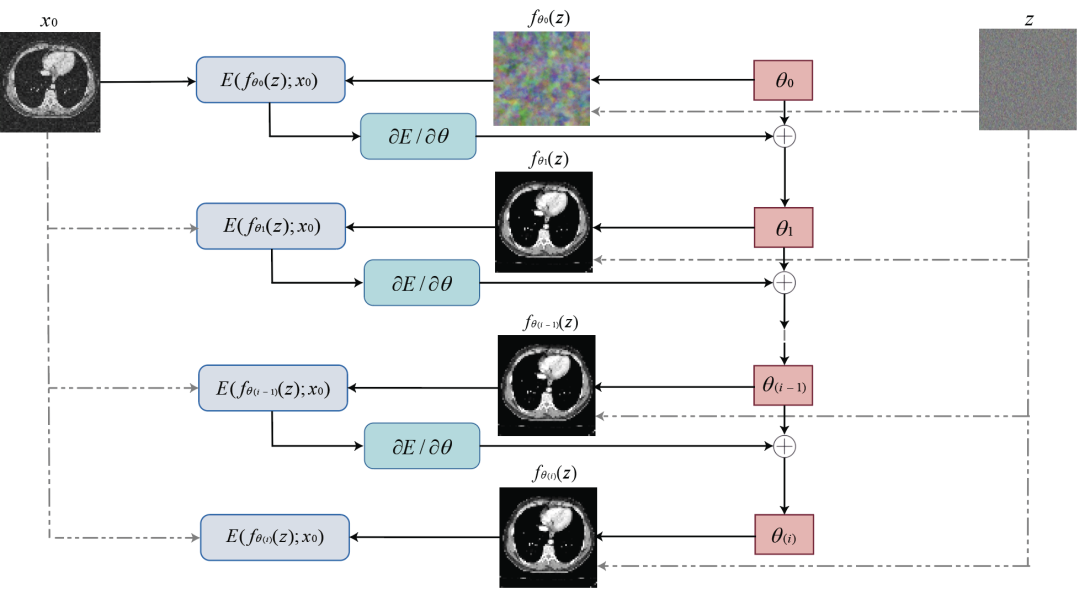
Figure 1: Network framework in image restoration.

3.2. Process

The images were output by the following steps:

10. The network weights were randomly initialised \( θ \) to generate an initial image \( {x=f_{θ}}(z) \) from a fixed random 3D tensor \( z \) .

11. \( θ \) was updated using gradient descent and other algorithms based on the energy function \( E({f_{θ}}(z);{x_{0}}) \) , where \( {x_{0}} \) is the input image.

12. \( θ \) was iteratively updated with the energy term \( E({f_{θ}}(z);{x_{0}}) \) using the same random 3D vector \( z \) until convergence.

13. The recovered image \( {f_{θ}}(z) \) was output when \( θ \) reached a local optimum, either when \( E({f_{θ}}(z);{x_{0}}) =0 \) or when the optimal stopping point was reached.

Details are included in the technical report [9].

3.3. Network with Resistance to High Noise

Although almost all images can be adapted to the network, the adaptation degree of low noise images and high noise images is different because the network architecture has selective retention of information. The neural network will resist the results that do not conform to the ground truth image and will decline in the direction of the ground truth, with the decline in efficiency of the natural image being higher.

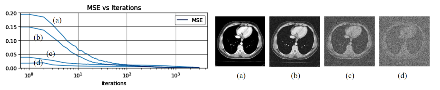
Figure 2: Learning curves for the reconstruction task using CT images with different levels of Gaussian noise.

In order to quantify the influence of different image noise intensity on the network reconstruction effect, we compared the distance \( {L^{2}} \) between the generated image and the input image \( {x_{0}} \) .

Figure 2 shows the energy \( E(x;{x_{0}}) \) and the iterative process under the selection of four different images: (a) a natural image, (b) the same image with Gaussian noise intensity of variance = 0.01, (c) the same image with Gaussian noise intensity of variance = 1, (d) the same image with Gaussian noise intensity of variance = 10.

From this image it can be seen that the network optimises the original image and the natural image with low noise intensity faster, while it has obvious resistance to strong noise. This reflects the characteristics of parameterisation: the retention of signal information is preferred over noise. According to this conclusion, for the actual image reconstruction problem, we limited the number of iterations to ensure that the model learning was focused on the signal information to reduce the sensitivity to noise and used the network internal regularisation to avoid noise overfitting.

3.4. Details in Applications

14. Denoising: Under the assumption of blind denoising, we used the same energy term as above. Given a CT image degraded due to complex and unknown compression artifacts, the restored clean image was output after substituting the minimised \( θ \) .

15. Super resolution: Super resolution is a problem of obtaining a higher resolution image from the reverse of the resolution image. We replaced the energy term with \( E(x;{x_{0}})={ ∥d(x)-{x_{0}}^{2}}∥ \) , where \( d(\cdot ) \) is a subsampler calculated by minimising the distance between the desired high-resolution image and the original image and using the subsampler in reverse. Regularisation was used at the same time to pick out the output image that best matches the expectation.

16. Inpainting: We replaced the energy term with \( E(x;{x_{0}})={ ∥(x-{x_{0}})⊙m∥^{2}} \) to measure the difference between the current image \( x \) and the missing part of the original image \( {x_{0}} \) . This was also used to transform the optimisation problem into the solution of the latent variable \( z \) , using \( z \) to indirectly affect the value of \( x \) to introduce the prior knowledge constraint solution.

17. Restoration: Restoration considers image restoration drawn according to a mask randomly sampled from a binary Bernoulli distribution. We sampled a mask and randomly dropped the pixels by 50%. In this case, the missing part of the image was repaired.

4. Experiment

In this experiment, we used a GPU (memory size of 15.0 GB), with system RAM of 12.7 GB and a disk size of 112.6 GB. The medical image data that was used came from two datasets of AI Studio website: CHAOS Multi-organ Segmentation dataset [10] and TCGA-LIHC Liver CT [11]. The CHAOS dataset includes 40 liver/spleen/kidney CT scans with segmentation labels, while the TCGA-LIHC Liver CT dataset comprises clinical images.

We applied the medical image data to the unsupervised deep learning model and optimised the algorithm, adjusted the learning rate, no.scales and other parameters to improve the model performance. Then, we obtained the optimal optimisation result by comparing the final PSNR value of different experimental parameters and the visual perception analysis of the output image.

A total of four image reconstruction tasks were completed. Following this, we summarised the results on a PSNR line chart and output result comparison chart. However, due to space limitations, we put two tasks in the technical report [9] and only described two tasks in the main body.

4.1. 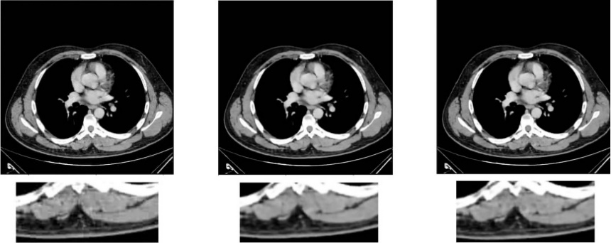Denoising

(a) (b) (c) (d)

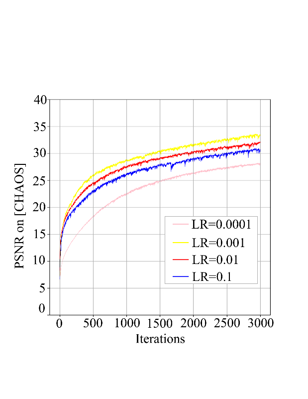
Figure 3: (a) Performance of denoising comparing different learning rates, (b) the original image, (c) output image when learning rate = 0.001, (d) output image when no.scale = 3.

In denoising application, we adjusted the values of learning rate {0.0001, 0.001, 0.01, 0.1} and no.scales {3, 4, 5, 6, 7} for the CHAOS dataset by means of control variables and evaluated the quality of output images with PSNR values.

In the process of adjusting the learning rate, we found that the learning rate of the original model was 0.01. Moreover, the output image displayed the best quality, even better than the original image, when it was exponentially reduced to 0.001, while the output image quality was not as good as the original when it was reduced to 0.001 or increased to 0.1.

In the process of adjusting the values of no.scales, we found the result was similar to that of adjusting the learning rate, where the output image quality would be the best when the no.scales was reduced to 3.

4.2. Inpainting

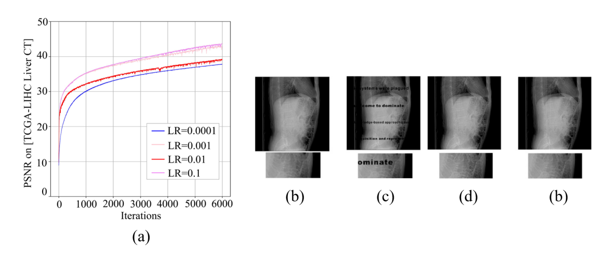
Figure 4: (a) Performance of inpainting comprising of different learning rates, (b) the original image; (c) the corrupted image, (d) output image when learning rate = 0.001, (e) output image when no.channels = 4.

In the inpainting application, we adjusted the values of the learning rate {0.0001, 0.001, 0.01, 0.1} and no.channels {3, 4, 5, 6, 7} for the TCGA-LIHC Liver CT dataset using the same method as denoising.

We found that the results of the adjustment were similar to the previous application, where the model works best when the learning rate was exponentially expanded to 0.1 from 0.01, which is the original value.

In the process of adjusting no.channels in inpainting application, we found that the original model no.channels was 5 and the output image displayed the best quality when it was reduced to 4, followed by the effect when it was expanded to 6 and 7, both of which were better than the original output results. However, the output image was poor when it was reduced to 3.

5. Conclusion

In this paper, we applied CT images to an unsupervised deep learning image reconstruction model and optimised the reconstruction results by changing the model parameters and hyperparameters. In future work, we will continue to optimise the restoration part and enhance the application range of CT image restoration.

References

[1]. Baguer, D. O., Leuschner, J. and Schmidt, M. (2020) Computed tomography reconstruction using deep image prior and learned reconstruction methods. Inverse Problems, 36(9), 094004.
[2]. Diwakar, M. and Kumar, M. (2018) A review on CT image noise and its denoising. Biomedical Signal Processing and Control, 42, 73-88.
[3]. Cui, J., Gong, K., Guo, N., Wu, C., Meng, X., Kim, K., ... and Li, Q. (2019) PET image denoising using unsupervised deep learning. European Journal of Nuclear Medicine and Molecular Imaging, 46, 2780-2789.
[4]. Umehara, K., Ota, J. and Ishida, T. (2018) Application of super-resolution convolutional neural network for enhancing image resolution in chest CT. Journal of digital imaging, 31, 441-450.
[5]. Park, J., Hwang, D., Kim, K. Y., Kang, S. K., Kim, Y. K. and Lee, J. S. (2018) Computed tomography super-resolution using deep convolutional neural network. Physics in Medicine & Biology, 63(14), 145011.
[6]. Peng, C., Li, B., Li, M., Wang, H., Zhao, Z., Qiu, B. and Chen, D. Z. (2020) An irregular metal trace inpainting network for x‐ray CT metal artifact reduction. Medical Physics, 47(9), 4087-4100.
[7]. Salem, N., Malik, H. and Shams, A. (2019) Medical image enhancement based on histogram algorithms. Procedia Computer Science, 163, 300-311.
[8]. Yamashita, K. and Markov, K. (2020) Medical image enhancement using super resolution methods. In Computational Science–ICCS 2020: 20th International Conference, Amsterdam, The Netherlands, June 3–5, 2020, Proceedings, Part V 20 (pp. 496-508). Springer International Publishing.
[9]. Yanchuan, Y. (2025) CT Image Reconstruction and Optimization with Unsupervised Deep Learning (Technical Report). https://github.com/YYC-CHUAN/dip-CTuse
[10]. CHAOS Multi-organ Segmentation dataset: https://aistudio.baidu.com/datasetdetail/23864
[11]. TCGA-LIHC Liver CT: https://aistudio.baidu.com/datasetdetail/37439
Cite this article
Yin,Y. (2025). CT Image Reconstruction and Optimisation with Unsupervised Deep Learning. Applied and Computational Engineering,118,95-100.
Data availability
The datasets used and/or analyzed during the current study will be available from the authors upon reasonable request.
Disclaimer/Publisher's Note
The statements, opinions and data contained in all publications are solely those of the individual author(s) and contributor(s) and not of EWA Publishing and/or the editor(s). EWA Publishing and/or the editor(s) disclaim responsibility for any injury to people or property resulting from any ideas, methods, instructions or products referred to in the content.
About volume
Volume title: Proceedings of the 3rd International Conference on Software Engineering and Machine Learning
© 2024 by the author(s). Licensee EWA Publishing, Oxford, UK. This article is an open access article distributed under the terms and
conditions of the Creative Commons Attribution (CC BY) license. Authors who
publish this series agree to the following terms:
1. Authors retain copyright and grant the series right of first publication with the work simultaneously licensed under a Creative Commons
Attribution License that allows others to share the work with an acknowledgment of the work's authorship and initial publication in this
series.
2. Authors are able to enter into separate, additional contractual arrangements for the non-exclusive distribution of the series's published
version of the work (e.g., post it to an institutional repository or publish it in a book), with an acknowledgment of its initial
publication in this series.
3. Authors are permitted and encouraged to post their work online (e.g., in institutional repositories or on their website) prior to and
during the submission process, as it can lead to productive exchanges, as well as earlier and greater citation of published work (See
Open access policy for details).