1. Introduction

Motor imagery EEG (MI-EEG) is a key area in the field of Brain-Computer Interface. MI signals are recorded when subjects imagine motioning without any physical action. The ipsilateral and contralateral motor perception cortexes exhibit event-related synchronization (ERS) and desynchronization (ERD) during such imagery, providing a physiological basis for EEG classification [1].

Over the past decade, the two most popular classifiers for EEG recognition have been Support Vector Machine (SVM) and Linear Discriminant Analysis (LDA) [2]. However, traditional studies faced challenges due to the low signal-to-noise ratio (SNR) of signals, resulted in low classification rates [3].

In the extant literature, research applies continuous wavelet transform (CWT) to convert original EEG data into time-frequency images to extract signal information. However, CWT does not perform well for MI signals due to their low frequencies. Compared with CWT, the short-time Fourier Transform (STFT) provides clear spectral identities in 8-30 Hz, and has low computational complexity, which outperforms CWT while transforming low-frequency MI-EEG signals into images with time-frequency identities.

Scientific deep-learning approaches such as Convolutional neural networks (CNN) have significantly increased the performance of image comprehension and classification [4]. CNN transcends the limitations of traditional machine learning networks, which rely on manually designed parameters to extract features. Besides, CNN enhances the ability to capture spatial features in images, thereby significantly improving the recognition and classification capabilities of EEG signals, especially for motor imagery signals [5]. Recent studies have proposed various CNN feature fusion architectures that integrate time-frequency information. For instance, dual-stream CNN (DCNN) models proposed by Huang et al.[6], apply both time and frequency-domain signals as inputs, using linear weighting for fusion to achieve end-to-end learning. This fusion of time-frequency features and CNN-based deep learning techniques opens a new feature fusion mechanism, offering improved recognition and control capabilities for MI-EEG applications.

However, DCNN does not explore temporal connections among features. Instead, it investigates features in different time periods separately, which is insufficient for discriminative feature extraction. We discovered that to increase the MI-EEG decoding efficiency, temporal relationships among MI-related patterns at different stages during MI tasks are crucial. As such, our goal is to create connections between features that were taken from various time periods. In recent years, generative models for image recognition have made extensive use of attention mechanisms. By assigning each context element an attention weight that defines a weighted sum across context representations, it is able to learn dependencies among them in an efficient manner. Inspired by the attention-based lightweight convolution [7], meanwhile considering the scarcity of EEG training data, a unique double-dimensional multi-scale CNN (DDMSCNN) with attention mechanism is proposed for MI-EEG classification in this paper.

We report methodology in Section 2, experimental findings in Section 3, discussions in Section 4, and conclusions in Section 5.

2. Methodology

In this section, we illustrate the procedure and details of our proposed network architecture. Fig.1 shows the overall structure of our hybrid model, where MSCNN is multi-scale CNN, which means having different scales of convolution kernels.

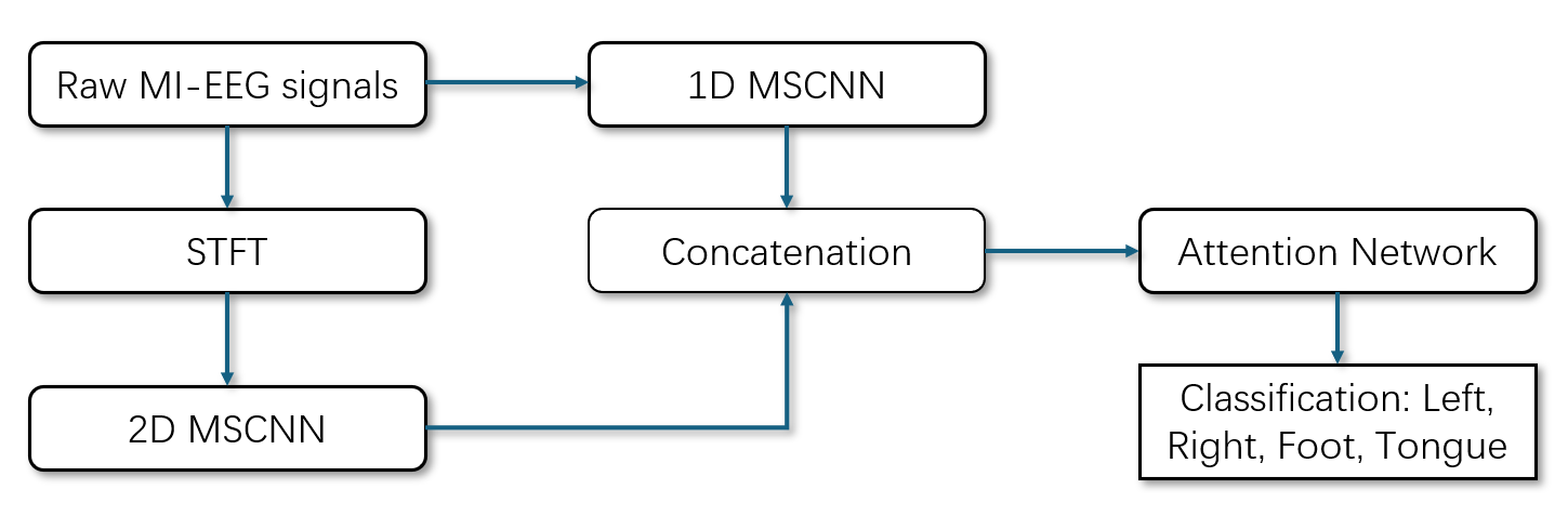
Figure 1. Structure of the proposed model.

The raw MI-EEG signals are processed through two branches. The signals in the first branch go straight via 1D-MSCNN. In the second branch, the signals are preprocessed using STFT before passing through 2D-MSCNN. The CNN outputs are concatenated and fed into the attention network to form the 4-class classification result.

2.1. Data Preprocessing

The BCI Competition IV dataset 2a is utilized for training and testing the proposed network to evaluate and improve performance [8]. The dataset was recorded with a sampling frequency of 250 Hz and 22 EEG channels. In this competition, nine patients performed four different motor imagery tasks: tongue (class 0), feet (class 1), right hand (class 2), and left hand (class 3) movements. Each patient participated in two sessions on different days, with measured data used for training (T) and validation (V), which resulted in a total of 18 files. Each session included six runs, and each run consisted of 48 trials (12 trials for each task).

During each trial, the patient faced a computer screen at ease. As shown in Fig.2, at the beginning of the trial (t=0s), a fixation cross appeared on the screen accompanied by a 70ms auditory cue. At t=2s, a prompt lasting about 1.25s appeared on the screen instructing the patient to perform motor imagery of the left hand, right hand, feet, or tongue. The EEG equipment captured the brain activity corresponding to the motor imagery and transmitted it to a computer. The patient continued the motor imagery until the fixation cross disappeared at t=6s. The screen then turned black, offering a rest period before the next trial.

The dataset includes labels, patient information, events, event markers, and recording times. We selected the dataset saved in .csv format and extracted signals from t=1.900s to t=2.700s, yielding a 0.800-second segment containing 200 samples. Thus, we obtained a data matrix set:

\( D=\lbrace [{X_{1}} {Y_{1}}], [{X_{2}}{ Y_{2}}],..., [{X_{22}} {Y_{22}}]\rbrace \)

where \( {X_{i}}∈{R^{200×2248}} \) , \( {Y_{i}}∈{R^{1×2248}} \) , 200 is the sample number of each trial, 2248 is the number of trials, and 22 is the number of channels. The input matrix of the \( {i^{th}} \) channel \( {X_{i}} \) contains 2248 trials, and each trial has 200 data samples. The matching label \( {Y_{i}}={({y_{1}} {y_{2}} ... {y_{2248}})^{T}} \) , where \( {y_{j}}∈\lbrace tongue: 0, foot:1, right hand: 2, left hand: 3\rbrace \) .

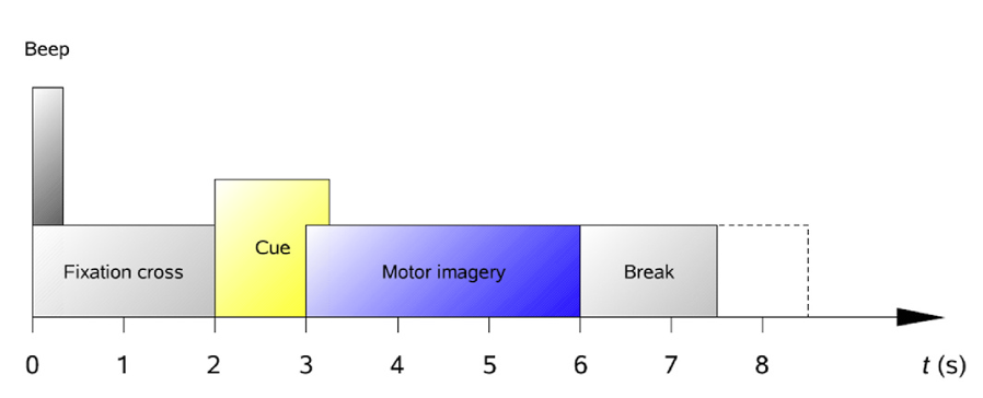
Figure 2. Timing scheme of each trial [8].

The cue appears on the screen at t=2s and last for 1.25s, instructing the patient to perform motor imagery of the left hand, right hand, feet, or tongue. The patient continued the motor imagery until the fixation cross disappeared at t=6s.

2.2. STFT

MI-EEG signals are inherently non-stationary, meaning their statistical properties change over time. A popular method to extract and demonstrate the frequency features of MI-EEG signals is the short-time Fourier Transform (STFT). This STFT algorithm transfers the 1D signal in the time domain to the 2D time-frequency domain image. STFT breaks the signal into short-time segments, applies the Fourier Transform to each segment, and observes their frequency characteristics. STFT can be represented by the following formula:

\( STFT\lbrace x(t)\rbrace (τ,f)=\int _{-∞}^{∞}x(t)∙w(t-τ)∙{e^{-j2πft}}dt \) (1)

where w(t) represents the window function, and x(t) represents the signal to transform. Apply proper window function, the raw MI-EEG signals can transform into 2D time-frequency images.

In our model, the input of the MI-EEG signal is a (200, 22) 2-D array. STFT will only operate the parameter in the time domain, which is “200”. For user-independent classification, applying window length 50 and hop size 25, we get the preprocessing result by STFT, which is a (26, 9, 22) 3-D array, providing a rich representation of the time-varying spectral content of the MI-EEG signals, making it suitable for subsequent analysis and model training. Fig.3 demonstrates the results of STFT transformation.

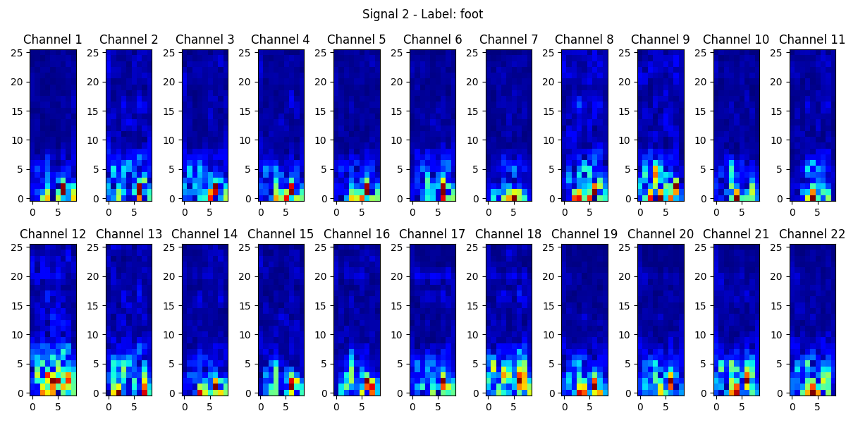
Figure 3. STFT images for the “foot” signal of each channel.

Colors from dark blue to red indicate the rise in the intensity of the specified frequency component in the time gap.

2.3. Double-Dimensional Multi-Scale CNN (DDMSCNN) Model

We constructed our CNN-based model, DDMSCNN, as shown in Fig.4. DDMSCNN contains a double-dimensional 1-D and 2-D CNN, each has three convolution layers. For user-independent classification, 1-D CNN contains convolution kernel sizes of 1 to 3, and 2-D CNN contains convolution kernel sizes of (1,1) to (3,3). Learning rate is set at 0.0010 and stride L=1. The following step is activation by the Exponential Linear Unit (ELU):

\( ELU(x)=\begin{cases} \begin{array}{c} α({e^{x}}-1), x \lt 0 \\ x , x≥0 \end{array} \end{cases} \) (2)

It outputs a minimum negative value for negative inputs, allowing the model to continue convoluting for critical negative input conditions. Both 1-D and 2-D CNN models applied Max pooling with a kernel scale of 2, highlighting the distinctive features and reducing the data sizes. The Dropout layer then eliminates overfitting at a dropout rate of 0.6, forcing the network to absorb robust features. Instead of applying a full-connection layer, we reshaped the output of 2-D CNN to match the dimensions of the 1-D CNN output to best preserve data features. The outputs are then concatenated linearly to form a 67 \( × \) 128 matrix as the output of DDMSCNN.

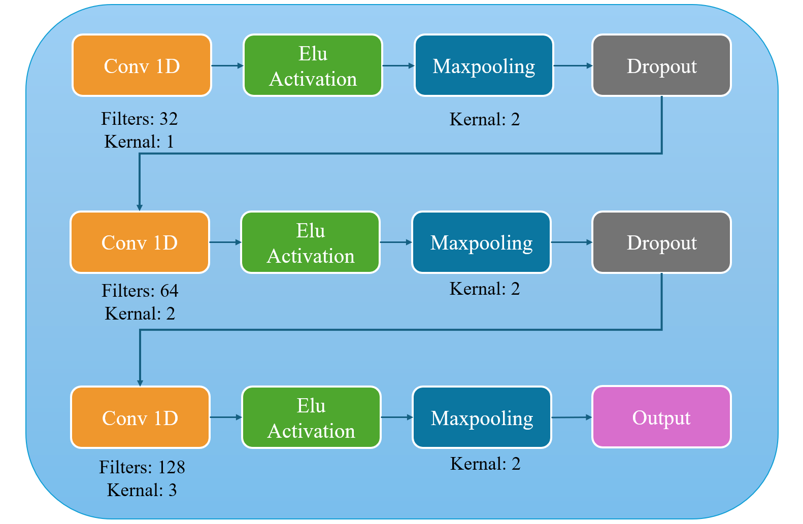
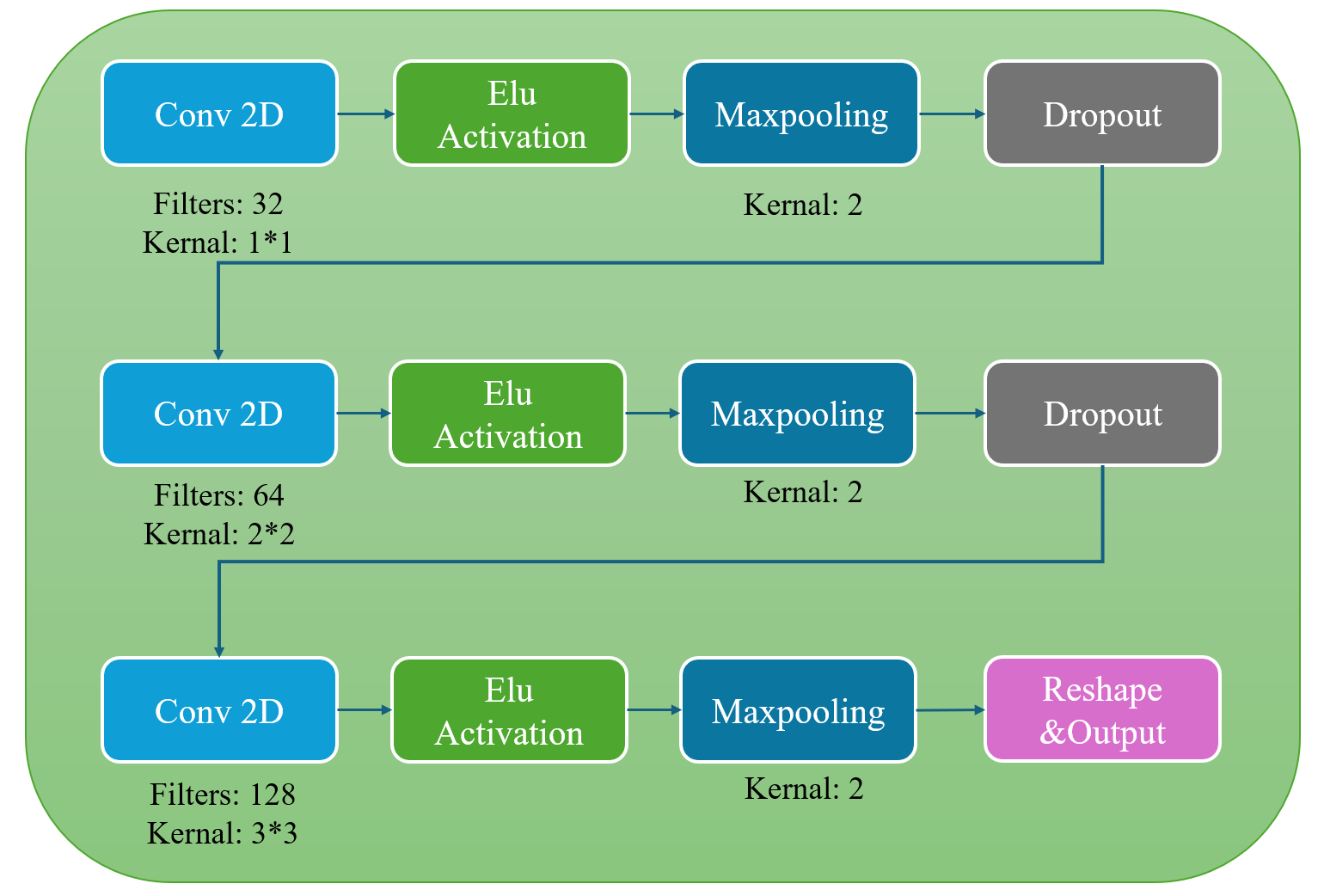
Figure 4. 1-D and 2-D CNN structures of DDMSCNN for user-independent classification.

The input is processed through convolution, ELU activation, max pooling and dropout. Three iterations of the procedure are carried out, incorporating modifications to the convolution filters and kernels.

2.4. Attention Module

The proposed attention network is designed to process the output matrix, which has a size of 67 \( × \) 128, from our DDMSCNN model. The structure of the attention network is shown in Fig.5. This network generates a weighted representation of the input feature maps within its first dense layer. This initial dense layer utilizes the "tanh" activation function for transforming the dense input and contains the same number of units as the two-dimensional input shape.

Subsequently, another dense layer, which has the activation function “softmax”, is employed to compute the attention weights. “Softmax” ensures the output forms a probability distribution across the feature maps. These weights are then reshaped into a vector with a size of 67 \( × \) 1.

Following this, the feature space from the input layer is element-wise multiplied by the reshaped attention weights, resulting in an output matrix of 67x128. This matrix is then flattened into a one-dimensional array of size 8576 \( × \) 1. Finally, this array is input into a final dense layer with a "softmax" activation function, producing the ultimate output of the network.

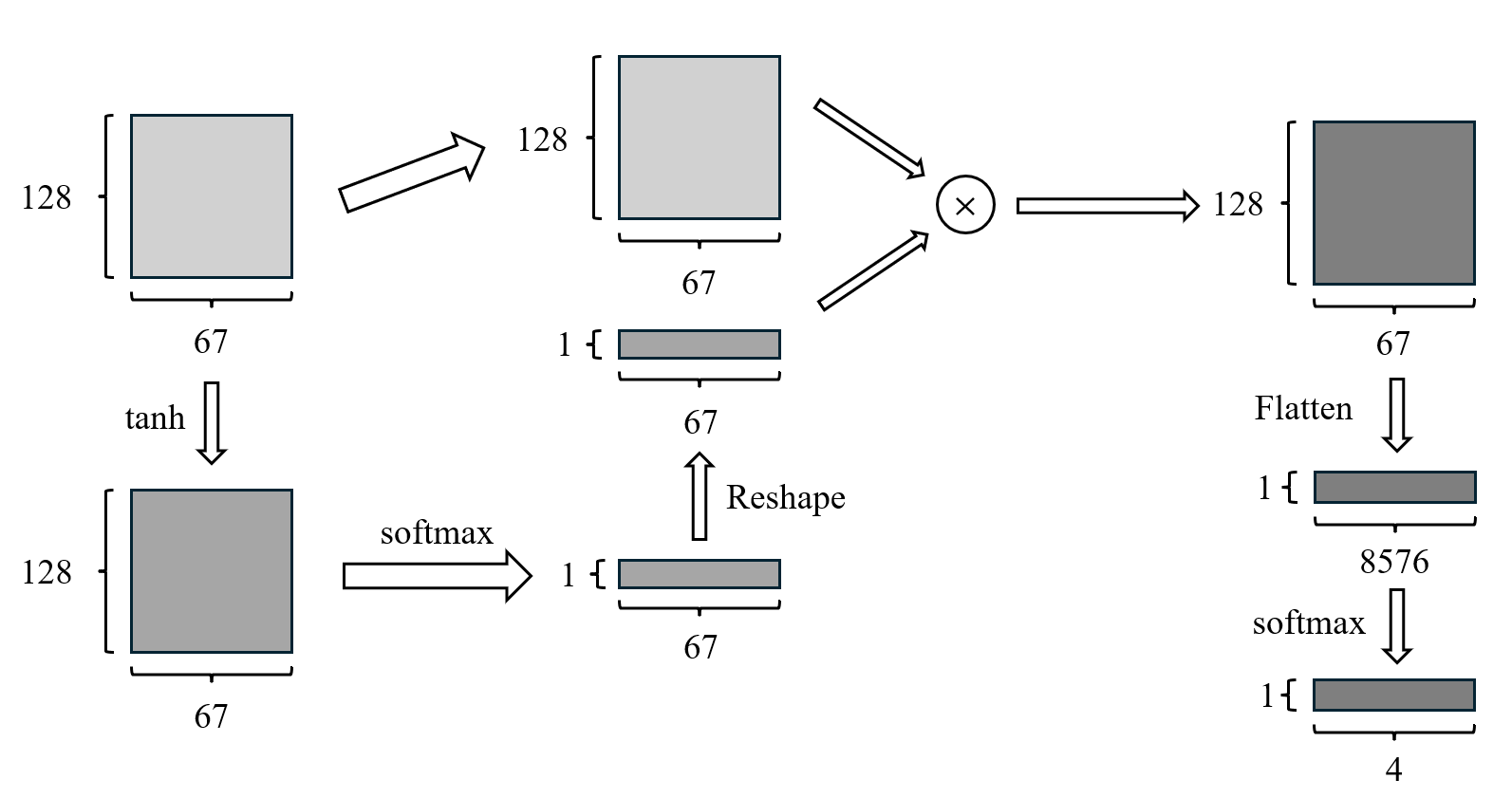
Figure 5. Structure of the attention module.

The initial dense layer utilizes the "tanh" activation function for transforming the dense input. The second dense layer with the activation function “softmax” is employed to compute the attention weights with a 67 \( × \) 1 vector. The input layer is element-wise multiplied by the reshaped attention weights, then flattened and inputted into a final dense layer with the "softmax" activation, producing the prediction of the classification task.

3. Results

3.1. Performance of the Proposed Network

The results of our study are summarized in Table 1, Fig.6 and Fig.7. As shown in Fig.6, despite the slight overfitting indicated by the disparity between training and testing accuracy, our hybrid model demonstrates stability. The validation loss remains low, and the model achieves average high accuracy, showing the feasibility and advancement of our approach.

Table 1. Performance of the proposed network.

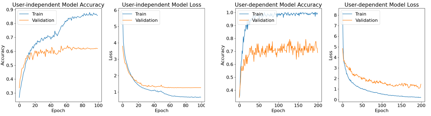
Figure 6. The accuracy and loss curve of the proposed network.

The user-independent accuracy has stabilized at 64%. The user-dependent result, derived from patient 7, has reached a peak of 79%.

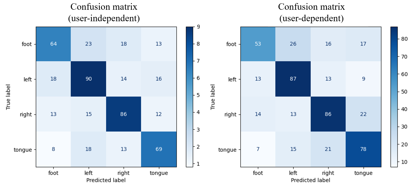
Figure 7. Confusion matrix of the proposed model.

The sum of each row in the matrix indicates the total number of epochs used for the actual test set of a specific category, while the sum of each column shows the total epochs classified for that category through the output layer. The unequal totals arise due to a break function in the network, which halts learning upon loss function convergence to save computational resources. Consequently, the capacity of the test sets varies.

3.2. Base-line Methods Performance Comparison

To evaluate the performance of our model, we make comparisons with related methods and classical deep-learning models. Table 2 provides the hyperparameter settings for user-dependent classification, while Table 3 presents the classification accuracy of baseline methods and our proposed approach. The hyperparameters for the 1D-CNN are specified as filters and kernels 1 to 3, whereas those for the 2D-CNN are indicated as filters and kernels 4 to 6. Filters 3 and 6 share the same parameters due to the concatenation of the CNN outputs. Consequently, filter 6 is not listed in Table 2.

Table 2. Hyperparameter settings of user-dependent classification.

Table 3. Classification accuracy of baseline methods and our method (%).

Our method has achieved high accuracy in user-dependent tests, outperforming all baseline methods. However, we observed variability in the user-dependent accuracies of our model. Specifically, apart from patient 4, whose data comprises only two classes, the highest classification accuracy was achieved with patient 5 at approximately 80%. Conversely, the lowest classification accuracy was recorded with patient 8, at only about 60%. These results indicate that our model is not fully effective in recognizing all patient data. Therefore, enhancing the adaptability of our model is crucial for future improvements.

4. Discussion

Without dividing the input data by time periods, our model successfully managed the 4-class classification, indicating the accomplishment of our requirement. Despite these improvements, optimization is still necessary due to the classification accuracy, memory consumption, and computational demand. We recognize that to reduce computational loads, model compression techniques like weight reduction and quantization are essential. While our model has demonstrated its classification abilities of MI-EEG, efficiency without sacrificing accuracy is still a goal. Future work will focus on refining the attention mechanism, exploring model compression, and incorporating advanced technologies to better capture the complex dynamics of MI-EEG signals. Our aim is to modify our model that ultimately reaches the performance of high accuracy and efficiency, thereby making practical application in real-world scenarios. Essentially, our findings highlight the potential of deep learning for MI-EEG classification, but also acknowledging the necessity for network optimization and the integration of advanced techniques to fully use the properties of MI-EEG signals.

5. Conclusion

In this study, we assessed the performance of our proposed hybrid model for MI-EEG signal classification, which integrates short-time Fourier Transform (STFT), Double-Dimensional Multi-Scale CNN (DDMSCNN), and an attention mechanism. Our method effectively overcomes the drawbacks of traditional CNNs in identifying MI-EEG features by incorporating multi-scale convolutions and the attention network that enhances the representational ability of the model. The addition of STFT transforms MI-EEG signals into 2-D time-frequency images, further improving recognition accuracy.

The experimental results show that our model achieves better performance than the baseline methods. The user-independent model achieved an accuracy of 64.04%, and the user-dependent model achieved an accuracy of 70.50%. The steadily high classification accuracy demonstrates the improvement in managing MI-EEG signals. Despite the promising outcomes, there are still challenges to be solved. The overfitting issue shows the necessity of model structure and hyperparameters modification, and the variability of user-dependent test results indicates user applicability enhancement. Future work will focus on minimizing overfitting, reducing computation load, and exploring additional techniques to enhance the model performance. In summary, our study offers a novel and effective network for MI-EEG signal classification, utilizing STFT, DDMSCNN, and attention mechanism. This research advances the field of EEG-based BCI, offering potential applications in neurorehabilitation and assistive technologies.

References

[1]. G. Pfurtscheller and F. L. da Silva, “C40EEG Event-Related Desynchronization and Event-Related Synchronization,” in Niedermeyer’s Electroencephalography: Basic Principles, Clinical Applications, and Related Fields, D. L. Schomer, F. H. Lopes da Silva, D. L. Schomer, and F. H. Lopes da Silva, Eds., Oxford University Press, 2017, p. 0. doi: 10.1093/med/9780190228484.003.0040.
[2]. A. Akrami, S. Solhjoo, A. Motie-Nasrabadi, and M.-R. Hashemi-Golpayegani, “EEG-Based Mental Task Classification: Linear and Nonlinear Classification of Movement Imagery,” Conf Proc IEEE Eng Med Biol Soc, vol. 2005, pp. 4626–4629, 2005, doi: 10.1109/IEMBS.2005.1615501.
[3]. F. Lotte et al., “A review of classification algorithms for EEG-based brain-computer interfaces: a 10 year update,” J Neural Eng, vol. 15, no. 3, p. 031005, Jun. 2018, doi: 10.1088/1741-2552/aab2f2.
[4]. J. Gu et al., “Recent advances in convolutional neural networks,” Pattern Recognition, vol. 77, pp. 354–377, May 2018, doi: 10.1016/j.patcog.2017.10.013.
[5]. R. R. Chowdhury, Y. Muhammad, and U. Adeel, “Enhancing Cross-Subject Motor Imagery Classification in EEG-Based Brain-Computer Interfaces by Using Multi-Branch CNN,” Sensors (Basel), vol. 23, no. 18, p. 7908, Sep. 2023, doi: 10.3390/s23187908.
[6]. E. Huang, X. Zheng, Y. Fang, and Z. Zhang, “Classification of Motor Imagery EEG Based on Time-Domain and Frequency-Domain Dual-Stream Convolutional Neural Network,” IRBM, vol. 43, no. 2, pp. 107–113, Apr. 2022, doi: 10.1016/j.irbm.2021.04.004.
[7]. F. Wu, A. Fan, A. Baevski, Y. N. Dauphin, and M. Auli, “Pay Less Attention with Lightweight and Dynamic Convolutions,” Feb. 22, 2019, arXiv: arXiv:1901.10430. doi: 10.48550/arXiv.1901.10430.
[8]. M. Tangermann et al., “Review of the BCI Competition IV,” Front. Neurosci., vol. 6, Jul. 2012, doi: 10.3389/fnins.2012.00055.
[9]. H. Bashashati, R. K. Ward, and A. Bashashati, “User-customized brain computer interfaces using Bayesian optimization,” J. Neural Eng., vol. 13, no. 2, p. 026001, Jan. 2016, doi: 10.1088/1741-2560/13/2/026001.
[10]. S. Sakhavi, C. Guan, and S. Yan, “Parallel convolutional-linear neural network for motor imagery classification,” in 2015 23rd European Signal Processing Conference (EUSIPCO), Nice: IEEE, Aug. 2015, pp. 2736–2740. doi: 10.1109/EUSIPCO.2015.7362882.
Cite this article
Sheng,H.;Wu,Q.;Chi,R.;Guo,Z. (2025). Time-Frequency Double-Dimensional Multi-Scale CNN with Attention Mechanism for Motor Imagery EEG Signal Classification. Applied and Computational Engineering,132,283-291.
Data availability
The datasets used and/or analyzed during the current study will be available from the authors upon reasonable request.
Disclaimer/Publisher's Note
The statements, opinions and data contained in all publications are solely those of the individual author(s) and contributor(s) and not of EWA Publishing and/or the editor(s). EWA Publishing and/or the editor(s) disclaim responsibility for any injury to people or property resulting from any ideas, methods, instructions or products referred to in the content.
About volume
Volume title: Proceedings of the 2nd International Conference on Machine Learning and Automation
© 2024 by the author(s). Licensee EWA Publishing, Oxford, UK. This article is an open access article distributed under the terms and
conditions of the Creative Commons Attribution (CC BY) license. Authors who
publish this series agree to the following terms:
1. Authors retain copyright and grant the series right of first publication with the work simultaneously licensed under a Creative Commons
Attribution License that allows others to share the work with an acknowledgment of the work's authorship and initial publication in this
series.
2. Authors are able to enter into separate, additional contractual arrangements for the non-exclusive distribution of the series's published
version of the work (e.g., post it to an institutional repository or publish it in a book), with an acknowledgment of its initial
publication in this series.
3. Authors are permitted and encouraged to post their work online (e.g., in institutional repositories or on their website) prior to and
during the submission process, as it can lead to productive exchanges, as well as earlier and greater citation of published work (See
Open access policy for details).