1. Introduction

The Density-Based Spatial Clustering of Applications with Noise [1] (DBSCAN) algorithm is a density-based clustering method that identifies clusters of arbitrary shapes by calculating mutual distances between data points without requiring any prior knowledge. DBSCAN constructs regions of high density and low density, making it particularly useful for anomaly detection. The algorithm clusters data based on two key parameters: the neighborhood radius Eps and the minimum number of points MinPts. The appropriate selection of these parameters is crucial for accurate clustering results. Current research on improving DBSCAN mainly focuses on tuning the parameters Eps and MinPts. Xia et al. [2] proposed an adaptive parameter determination method that calculates the statistical properties of the data. This method employs the inverse Gaussian distribution to identify the radius Eps corresponding to the peak point, and uses the inflection point of the noise curve to determine the minimum score MinPts within the radius, achieving adaptive parameter tuning. However, this approach performs poorly with high-dimensional data, has high computational complexity, and is time-consuming. Lei et al. [3] utilized sample silhouette coefficients and cluster silhouette coefficients to compare multiple sets of parameters and select the most effective parameters for clustering. The sample silhouette coefficient is calculated as follows: \( {s_{i}}=\frac{{∂_{i}}-{a_{i}}}{*max({a_{i}},{b_{i}})} \) , \( {s_{i}} \) ∈[−1,1]. Based on this, it can be determined whether a given sample fits its assigned cluster. The closer the value is to 1, the more appropriate the clustering. The cluster silhouette coefficient is defined as: \( {s_{k}}≡\frac{1}{n}\sum _{i=1}^{n}{s_{i}} \) . The silhouette coefficient for the entire dataset is the average of all sample silhouette coefficients. However, this approach still does not go beyond the scope of parameter tuning and fails to incorporate the unique data distribution characteristics inherent to power curves.

Li et al. [4] used DBSCAN as the base model and designed two evaluation metrics, prediction error and classification accuracy, to achieve fully automated selection of two clustering parameters: the neighborhood radius and the minimum number of samples in a neighborhood. However, the prediction error requires normal data to create both the training and testing datasets, while classification accuracy requires both normal and abnormal data for training, which is logically contradictory.

YaoQ et al. [5] introduced a mechanistic model, specifically the wind turbine power characteristic curve. Using the formula \( {P_{m}}=0.5πρ{R^{2}}{C_{p}}(λ,β){ν^{3}} \) , they calculated the minimum distance between the operational data and the theoretical model to dynamically adjust Eps and MinPts. Although this method incorporates the power characteristic curve, it does not integrate it holistically. Instead, it uses the characteristic formula solely to determine the relative distance from the characteristic curve, thereby setting the two parameters.

Hu [6] proposed a multi-density adaptive parameter determination algorithm. This approach generates candidate lists of Eps and MinPts parameters based on the distribution characteristics of a denoised and attenuated dataset. It selects corresponding Eps and MinPts values from the interval where the number of clusters stabilizes, using denoising levels as a reference. A distance distribution matrix is generated and sorted, with a decay term added during Eps determination: \( {Eps_{k}}=(1-{λ^{2}})\bar{{D_{k}}} \) , \( Ep{s_{-}}list=\lbrace Ep{s_{K}}|1⩽K⩽n\rbrace \) . However, for large-scale datasets, its time and space complexity can become prohibitive.

Zheng et al. [7] proposed a QM-DBSCAN-based data cleaning method. First, they applied the quartile method to clean wind speed-power data laterally. Next, they divided the cleaned data into wind speed intervals of 0.5 m/s, applying the DBSCAN method to determine the Eps and MinPts values for each interval and perform clustering. Compared with the traditional quartile and DBSCAN methods, their approach improved the correlation coefficient of the clustered data and achieved better cleaning results. However, it did not account for the mechanistic model of wind turbines.

In summary, although current improvements partially address the parameter selection problem of the DBSCAN model, manual intervention is still required to set certain parameter values. Furthermore, the distribution characteristics of wind turbines’ power-speed curves have not been integrated into existing anomaly detection methods.

Based on this, this study proposes a new method founded on the traditional DBSCAN algorithm. By introducing the distribution characteristics of the data to determine the clustering propagation direction and applying the 3σ criterion to adaptively determine Eps and MinPts, this method achieves full automation of the clustering process. The proposed method’s effectiveness is validated using operational data from actual production processes.

2. A DBSCAN-Based Anomaly Data Processing Method Driven by Data Distribution

The basic idea of this algorithm is to analyze the distribution characteristics of the data and incorporate these characteristics to redefine the clustering propagation direction. Unlike traditional density-based clustering algorithms, which expand clusters in spherical directions, this method adjusts the clustering propagation direction to align with the variations in data distribution. Using the 3σ criterion, parameters Eps and MinPts are determined for each data point, yielding the clustering results. The DBSCAN algorithm is then applied to label data points with insufficient density as anomalies, resulting in the final anomaly detection outcomes.

2.1. The DBSCAN Algorithm

The DBSCAN algorithm begins by selecting a data point as the starting point and calculating the density of all points within its neighborhood. If the density equals or exceeds a predefined threshold, the point is identified as a core point [8]; otherwise, it is classified as a noise point. For each core point, a neighborhood radius Eps is used to calculate the density of all points in its neighborhood. If the density meets or exceeds the threshold, these points are grouped into a cluster. For each border point, if it lies within the neighborhood of a core point, it is assigned to the cluster of that core point; otherwise, it is considered a noise point. Ultimately, all data points assigned to clusters constitute the clustering results, while noise points are identified separately as noise outcomes.

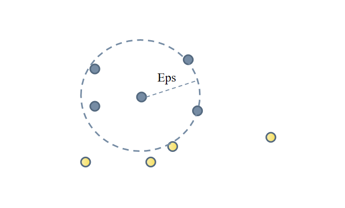
Figure 1: Schematic Diagram of the DBSCAN Algorithm

Definition: Eps Neighborhood

For any given data object \( p \) , its Eps neighborhood is defined as a multidimensional hypersphere space \( D \) , centered on \( p \) with a radius of Eps, where any object satisfies:

\( {N_{Eps}}(p)=\lbrace q∈D∣Dist(p,q)≤Eps\rbrace \)

Here, \( D \) represents the dataset in a multidimensional real space, and \( Dist(p,q) \) denotes the distance between data objects \( q \) and \( p \) in \( D \) .

Although DBSCAN inherently does not require pre-specifying the number of clusters and supports clustering of arbitrary shapes, its application has some limitations:

(1) Difficulty in Selecting Density Threshold and Neighborhood Radius: Proper selection of the density threshold and neighborhood radius requires adjustment based on the dataset’s characteristics. Inappropriate values may result in clusters with incorrect numbers or sizes.

(2) Poor Handling of Unevenly Distributed Data: DBSCAN struggles with datasets where density is uneven. Dense clusters may be split into multiple clusters, while sparse clusters may be misclassified as noise points.

2.2. DBSCAN Algorithm Driven by Data Distribution

2.2.1. The 3σ Criterion

The 3σ criterion, also known as the Lyida Criterion, is a data processing method used to identify and exclude outliers. Based on the assumption of a normal distribution, it calculates the standard deviation to establish an interval, treating errors beyond this range as anomalies and excluding them.

(1) Define the sample dataset \( X={x_{1}}{,x_{2}},{x_{3}},…,{x_{i}},i=1,2,3…n \)

(2) Compute the mean: \( m=\frac{1}{n}\sum _{i=1}^{n}{x_{i}} \)

(3) Calculate the standard deviation: \( σ=\sqrt[]{\frac{1}{n}}\sum _{i=1}^{n}({x_{i}}-m{)^{2}} \)

(4) Establish the confidence interval using the formula \( (m-3σ,m+3σ) \) , and exclude data points in \( X \) outside this range to obtain standardized data.

2.2.2. DBSCAN Clustering Algorithm Based on Data Distribution Features

The core idea of this algorithm is to introduce a mechanistic model to determine the specific shape of the data distribution [9]. Unlike traditional density-based clustering algorithms that expand clusters in spherical directions, this approach aligns the clustering propagation direction with the data’s variation direction. Using the 3σ criterion, it determines the parameters Eps and MinPts for each data point, ultimately obtaining the clustering results.

Assumptions:

Let the dataset \( X=({x_{1}},{x_{2}},,,…,{x_{k}}) \) represent k-dimensional vectors acquired by the SCADA system.

Propagation Direction:

The clustering propagation direction is determined along the specific distribution of the mechanistic model. Assuming the data at time t is \( {x^{t}} \) , the propagation direction is expressed as:

\( {Dir_{B}}=\frac{∂P}{∂{x^{t}}}=(\frac{∂P}{∂1_{t}^{x}},\frac{∂P}{∂2_{t}^{x}},,,…,\frac{∂P}{∂k_{t}^{x}}) \) (1)

By comparing the cosine similarity between the gradient changes of data within the neighborhood radius Eps and the propagation direction, a threshold Threshold is set. Points with a similarity score exceeding the threshold are assigned scores. Points with scores greater than Minpts are identified as core points. Starting from any core point, all density-reachable objects from this point form a cluster.

2.3. DBSCAN Anomaly Detection Method Driven by Data Distribution

The traditional DBSCAN algorithm involves two key custom parameters that significantly impact the classification results. The algorithm proposed in this paper emphasizes the necessity of incorporating data distribution characteristics, utilizing gradient variations in the data, and applying the statistical 3σ criterion to determine the values of Eps and MinPts [10]. Based on the theoretical model introduced in the previous section, the DBSCAN anomaly detection algorithm driven by data distribution (DD-DBSCAN) is described as follows:

Computational Steps:

a. Calculate the parameters Eps and MinPts. Randomly select any data point \( {x_{i}} \) , set the step size for data partitioning, and choose the data within the corresponding interval.

b. Using the normal distribution characteristics of the data, compute the mean ( \( {mean_{i}} \) ) and standard deviation ( \( {stdv_{i}} \) ) for the regional data. Based on the 3σ criterion, determine the confidence interval and filter out anomalous data.

c. Set the standard deviation σ of the corresponding interval as Eps, and define MinPts as the number of data points in the interval whose direction of change aligns with the clustering propagation direction, with an angle smaller than Threshold. The Threshold can be manually specified.

d. For each point, calculate the number of data points within the corresponding Eps neighborhood that conform to the specific direction, and compare this number with MinPts. If the number exceeds MinPts, classify the point as a normal point; otherwise, treat it as an anomalous point.

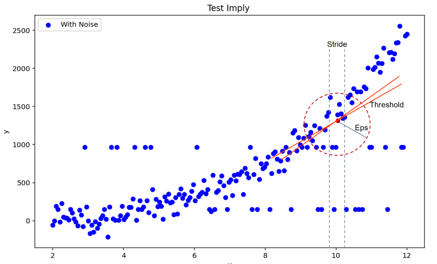
Figure 2: Schematic Diagram of Anomaly Detection Using the DD-DBSCAN Algorithm

3. Case Study

To better demonstrate the algorithm proposed in this paper, two test datasets, each containing 1000 two-dimensional data points, were used. As shown in Figure 3, the distribution of these 1000 two-dimensional data points can be observed. Unlike traditional test datasets where there is a large distance and separation between clusters, this test dataset contains mixed data distributions. In this case, a comparative experiment with the traditional DBSCAN algorithm was conducted [11], measuring the results from three dimensions: anomaly detection, running time, and recognition accuracy. The experimental environment used the Anaconda platform, with Python 3.12.1 as the programming language, and the hardware conditions were 256 GB SSD + 16 GB RAM + M4.

In this test, the dataset contains some noise points mixed in with the normal data. The traditional DBSCAN algorithm, which is based on density, can only utilize the density within the neighborhood radius and cannot distinguish the distribution of normal data. As seen in Figure 4, the method proposed in this paper can identify high-density regions within the dataset and make appropriate cluster divisions as desired, thereby detecting the noise points in the data.

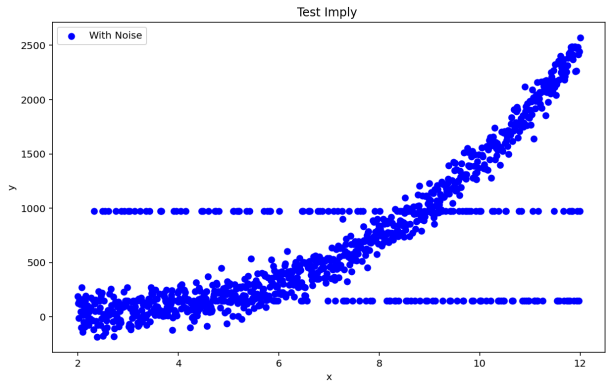
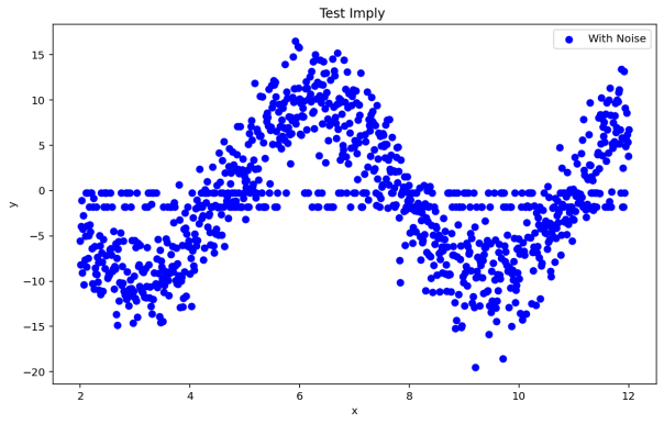
Figure 3: DS1 and DS2 Data Distribution

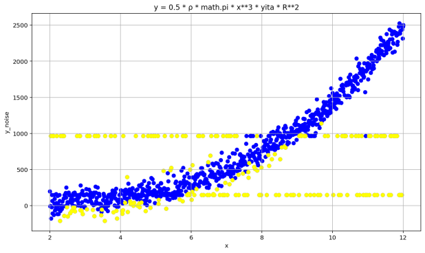
Figure 4: DD-DBSCAN Clustering Results for DS1 and DS2

The DBSCAN algorithm uses the R* tree extension algorithm for searching, with a time complexity \( O( nlog n \) ). The time complexity of the R* tree extension algorithm mainly comes from calculating distances between objects and k-nearest neighbors. In DBSCAN, the distance matrix already includes these calculations, so they do not need to be recalculated during the clustering process. However, compared to DBSCAN, SA-DBSCAN incurs two additional time costs:

The 3σ criterion is applied to each data point to compute the values of Eps and MinPts.

For each neighborhood radius, the number of data points within that interval whose direction of change has an angle smaller than the Threshold with the clustering propagation direction must be calculated.

We use the supervised F Measure method [12] to detect the clustering accuracy. The clustering results and accuracy metrics for the DS1 and DS2 datasets are shown in Table 1. For comparison, traditional DBSCAN clustering was also performed on the datasets. The DBSCAN parameters were selected using the K-dist graph to determine the optimal values, but due to space limitations, the clustering results for traditional DBSCAN are not shown.

Table 1: Comparison of Algorithm Computation Time and Clustering Accuracy

As shown in Table 1, in terms of time performance, SA-DBSCAN is indeed slower than DBSCAN due to the additional computation. However, there is no significant difference in the order of magnitude between the computation times of SA-DBSCAN and DBSCAN. Furthermore, since the clustering process is still the same as DBSCAN, any optimization made to DBSCAN can also improve the performance of SA-DBSCAN. Additionally, in terms of accuracy, the algorithm demonstrates better performance when handling datasets with non-spherical clusters (DS1, DS2). It can effectively handle datasets of any shape and identify anomalous data mixed within them.

4. Conclusion

The DBSCAN anomaly detection method driven by data distribution, proposed in this paper, successfully adapts the parameters of the DBSCAN algorithm by incorporating data distribution features and the 3σ criterion, improving the accuracy and automation of anomaly detection. The experimental results show that this method performs excellently when handling complex datasets, effectively identifying anomalies mixed with normal data, with significantly higher accuracy compared to the traditional DBSCAN algorithm. Future research can further optimize the time complexity of the algorithm and explore its performance in more practical application scenarios.

References

[1]. Ester, M. (1996). A density-based algorithm for discovering clusters in large spatial databases with noise. Proceedings of the International Conference on Knowledge Discovery & Data Mining.
[2]. Xia, L., & Jing, J. (2009). SA-DBSCAN: An adaptive density-based clustering algorithm. Journal of the University of Chinese Academy of Sciences, 26(4), 530-538. https://doi.org/10.7523/j.issn.2095-6134.2009.4.015
[3]. Lei, M., Guo, P., & Liu, B. (2021). Research on anomaly data identification for wind turbine units based on the adaptive DBSCAN algorithm. Journal of Power Engineering, 41(10), 859-865. https://doi.org/10.19805/j.cnki.jcspe.2021.10.007
[4]. Li, T., Wang, R., & Gao, J. A method for identifying SCADA anomaly data in wind turbine units based on improved DBSCAN. Journal of Xi’an Jiaotong University. Retrieved from [journal URL]
[5]. Yao, Q., Hu, Y., Liu, J., et al. (2023). Power curve modeling for wind turbines using a hybrid-driven outlier detection method. Journal of Modern Power Systems and Clean Energy, 11(4), 1115-1125.
[6]. Hu, D., Jiang, Y., & Wan, J. (2022). Research on an algorithm for determining DBSCAN parameters with multiple densities. Computer Engineering and Applications, 58(2), 8. https://doi.org/10.3778/j.issn.1002-8331.2012-0476
[7]. Zheng, Y., Liu, Y., He, Z., et al. (2021). Data cleaning method for wind turbine data based on QM-DBSCAN. Journal of Lanzhou University of Technology, 47(6), 6. https://doi.org/10.3969/j.issn.1673-5196.2021.06.009
[8]. Ankerst, M., Breunig, M. M., Kriegel, H. P., et al. (1999). OPTICS: Ordering points to identify the clustering structure. In Proceedings of the ACM SIGMOD International Conference on Management of Data (pp. 49-60). ACM. https://doi.org/10.1145/304182.304187
[9]. Li, W., & Xing, K. (2024). A data distribution-driven small-sample gradient-free learning method for sentiment classification. Electronics Technology, 3, 61-65.
[10]. Zou, T., Gao, Y., Yi, H., et al. (2020). Wind power anomaly data processing based on Thompson tau-quartile and multi-point interpolation. Automation of Electric Power Systems, 15, 10. https://doi.org/10.7500/AEPS20191231003
[11]. Li, W., Yan, S., & Jiang, Y. (2019). Research on an algorithm for adaptively determining DBSCAN algorithm parameters. Computer Engineering and Applications, 55(5), 1-7+148.
[12]. Steinbach, M., Karypis, G., & Kumar, V. (2000). A comparison of document clustering techniques. Journal of Data Mining and Knowledge Discovery, 3(4), 421-444.
Cite this article
Cui,H. (2025). A DBSCAN Anomaly Data Identification Method Driven by Data Distribution. Applied and Computational Engineering,108,156-162.
Data availability
The datasets used and/or analyzed during the current study will be available from the authors upon reasonable request.
Disclaimer/Publisher's Note
The statements, opinions and data contained in all publications are solely those of the individual author(s) and contributor(s) and not of EWA Publishing and/or the editor(s). EWA Publishing and/or the editor(s) disclaim responsibility for any injury to people or property resulting from any ideas, methods, instructions or products referred to in the content.
About volume
Volume title: Proceedings of the 5th International Conference on Signal Processing and Machine Learning
© 2024 by the author(s). Licensee EWA Publishing, Oxford, UK. This article is an open access article distributed under the terms and
conditions of the Creative Commons Attribution (CC BY) license. Authors who
publish this series agree to the following terms:
1. Authors retain copyright and grant the series right of first publication with the work simultaneously licensed under a Creative Commons
Attribution License that allows others to share the work with an acknowledgment of the work's authorship and initial publication in this
series.
2. Authors are able to enter into separate, additional contractual arrangements for the non-exclusive distribution of the series's published
version of the work (e.g., post it to an institutional repository or publish it in a book), with an acknowledgment of its initial
publication in this series.
3. Authors are permitted and encouraged to post their work online (e.g., in institutional repositories or on their website) prior to and
during the submission process, as it can lead to productive exchanges, as well as earlier and greater citation of published work (See
Open access policy for details).