1. Introduction

With the acceleration of global urbanisation, traffic congestion has become a core problem of modern urban governance. According to statistics, the economic loss caused by traffic congestion in major cities around the world is up to billions of dollars, while the accompanying tailpipe emissions exacerbate environmental pollution and energy consumption [1]. In this context, Intelligent Transport Systems (ITS), as a key technology to alleviate traffic pressure, relies on the accurate prediction of traffic flow as its core function. Traffic flow prediction provides decision support for traffic signal control, route planning, and accident early warning by analysing historical and real-time data and inferring the vehicle traffic status of a specific time and road section in the future. However, traffic flow has a high degree of nonlinearity and spatial and temporal correlation, and is affected by multiple factors such as weather, emergencies, holidays, etc. Traditional prediction methods are often difficult to capture complex data patterns, and there is an urgent need for more efficient and adaptive technological means [2].

Early traffic flow prediction was mainly based on statistical models and physical simulation. For example, the autoregressive integral sliding average model (ARIMA) captures the cyclical characteristics of traffic flow through time series analysis, and Kalman filtering is used to dynamically update the prediction results. In addition, simulation models based on traffic flow theory (e.g., VISSIM) generate forecast data by simulating vehicle micro-behaviour. However, these methods have significant drawbacks: statistical models rely on linear assumptions and cannot deal with nonlinear interactions in the traffic system; simulation models need to preset complex parameters and are computationally expensive, making it difficult to respond to the demands of large-scale road networks in real time. With the exponential growth of the amount of urban traffic data, the limitations of traditional methods become more and more prominent [3].

In recent years, deep learning has achieved breakthroughs in the field of traffic flow prediction through multi-layer neural network architectures. Convolutional neural networks (CNNs) are good at extracting spatial features of road network topology, e.g., transforming urban road networks into raster images to capture the traffic propagation patterns of adjacent road sections; recurrent neural networks [4] (RNNs) and their variants (e.g., LSTMs, GRUs) are capable of modelling long term dependencies in the temporal dimension, e.g., identifying sudden changes of the traffic pattern in the morning and evening peaks. To further incorporate spatio-temporal properties, researchers propose hybrid models such as CNN-LSTM [5] to capture spatio-temporal correlations simultaneously through joint training. In this paper, we optimise the long and short-term memory network based on time-domain convolutional network for traffic flow prediction and verify the effectiveness of the model through experiments.

2. Sources of data sets

This experiment uses open source dataset, the source of the dataset is kaggle, the dataset records the traffic flow of the road traffic over a period of time, containing the date, the number of cars passing, the number of bikes passing and the number of trucks passing. We choose 387 of these data for the experiment.

Table 1: Results of ablation experiments.

The graphs of changes in traffic flow for cars, bicycles and trucks are output separately, the graphs of changes in traffic flow for cars are shown in Fig. 1, the graphs of changes in traffic flow for bicycles are shown in Fig. 2 and the graphs of changes in traffic flow for trucks are shown in Fig. 3.

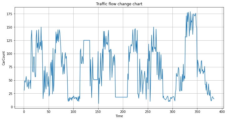
Figure 1: The graphs of changes in traffic flow for cars.

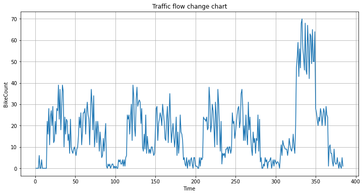
Figure 2: The graphs of changes in traffic flow for bicycles.

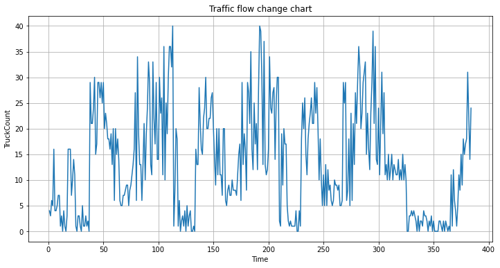
Figure 3: The graphs of changes in traffic flow for trucks.

3. Method

3.1. Time Domain Convolutional Networks

Time domain convolutional network (TCN) is a deep learning model designed specifically for time series data, and its core idea is to improve the structure of traditional convolutional neural network (CNN) by improving the structure of CNN, so that it can effectively capture long-range dependencies in the time dimension, and at the same time, overcome the limitations of recurrent neural network (RNN)-like models in terms of parallel computation and training efficiency [6]. The time domain convolutional network. The model structure diagram of the TCN is shown in Fig. 4.

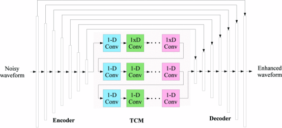
Figure 4: The model structure diagram of the TCN.

The core structure of TCN is based on causal convolution and dilation convolution. Causal convolution ensures that the model relies only on the input data of the current and past moments when predicting the output of the current time step, avoiding the leakage of future information, a feature that makes it naturally suitable for time series prediction tasks. Expansion convolution, on the other hand, can significantly expand the sensory field while keeping the number of parameters constant by introducing an ‘expansion factor’ to control the interval sampling of the convolution kernel. For example, the dilation factor grows exponentially as the number of network layers deepens, allowing the deeper network to capture earlier temporal features. This design allows TCNs to avoid the gradient vanishing problem of RNNs while being more efficient than traditional CNNs when dealing with long sequences [7].

To improve the depth and stability of the model, TCNs are usually combined with residual connectivity. Each residual block consists of multilayer dilated causal convolution and nonlinear activation functions, and passes the input directly to the output through jump connections. This structure not only mitigates the gradient vanishing problem, but also allows the network to learn the residual mapping between inputs and outputs to build deeper network structures. The stacking of residual blocks allows the model to extract features on different time scales layer by layer, ultimately fusing multiple levels of temporal information.

3.2. Long Short-Term Memory Networks

Long Short-Term Memory Network (LSTM) is a deep learning model designed to overcome the shortcomings of traditional Recurrent Neural Networks (RNNs), and is specifically designed to deal with long-term dependency problems in sequential data. In traditional RNNs, as the time step increases, it is difficult for the network to effectively deliver early information (i.e., there is a gradient disappearance or explosion), while LSTM achieves fine-grained control of the information by introducing a unique ‘memory unit’ and gating mechanism, which can both capture short-term features and maintain long-term memory.

The core design of LSTM is the ‘cell state’, which acts as a backbone through time and is responsible for the stable transmission of key information between different time steps. The stability of the cell state is regulated by three gating structures: the forgetting gate, the input gate and the output gate. These gates are not physical structures, but rather ‘switches’ modelled by neural network layers and activation functions that determine the retention or discard of information [8]. The structural schematic of the long and short-term memory network is shown in Figure 5.

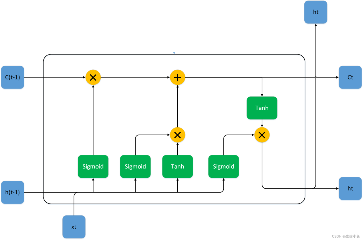
Figure 5: The structural schematic of the long and short-term memory network.

The forgetting gate is responsible for filtering historical information. It will determine which old information in the cell state needs to be retained or forgotten based on the current input and the hidden state of the previous moment [9]. The input gate, on the other hand, is responsible for filtering new information, and it combines the current input and the hidden state to determine which new features need to be integrated into the cell state. This process is similar to the ‘selective updating’ of human memory, which ensures that memory cells are always relevant to the current task. The output gate ultimately determines the current moment's output, which generates an externally visible prediction or feature representation based on the updated cell state and hidden state [10].

3.3. Long and short-term memory network based on time domain convolutional network optimisation

Time domain convolutional network (TCN) is an improved sequence modelling method based on convolutional neural network (CNN), which can effectively optimize the shortcomings of long short-term memory network (LSTM) in long sequence modelling by introducing mechanisms such as causal convolution and dilation convolution. The combination of the two mainly improves the model's ability to model time-series data in terms of structural complementarity and computational efficiency.

The shortcoming of LSTM is the order dependency due to its recursive structure: the computation of each time step must wait for the output of the previous moment, which limits the parallelism and may still face gradient decay in very long sequences. TCN circumvents this problem through causal convolution - its convolution kernel only allows access to the historical information at the current moment and does not involve the future data. future data, which preserves temporal causality and directly expands the sensory field by stacking multiple layers of dilated convolutions.

In addition, TCN's parameter sharing mechanism significantly reduces the number of parameters, alleviating the overfitting problem of LSTM due to the complex gating structure.

The optimisation of TCN for LSTM is mainly reflected in two aspects:

1. Parallel computation acceleration: the recursive computation of LSTM is naturally difficult to parallelise, while the convolutional operation of TCN can process the whole sequence at once, which significantly reduces the training time, especially in the GPU environment.

2. Explicit long-range dependency capture: LSTM relies on cell states to convey long-term information, but ultra-long sequences may still lead to ‘overloading’ of memory cells. TCN exponentially expands the sense field through residual concatenation and dilation convolution, explicitly covering a history window of thousands of time steps.

4. Experiments and Results

This experiment is divided into three groups: car traffic prediction, bicycle traffic prediction and truck traffic prediction. The experimental results of car traffic prediction are output first. The change of loss during the training process is shown in Fig. 6, the predicted-actual value scatter plot of the training set is shown in Fig. 7, and the predicted-actual value scatter plot of the test set is shown in Fig. 8, and the prediction of the future traffic is made by using the trained model, as shown in Fig. 9.

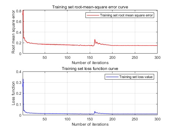
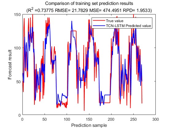
Figure 6: The change of loss. Figure 7: The predicted-actual value scatter plot.

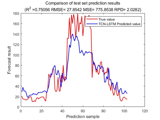
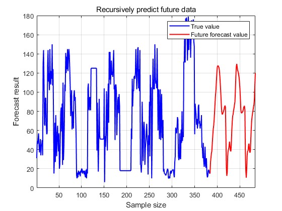
Figure 8: The predicted-actual value scatter plot. Figure 9: The prediction of the future traffic.

From the car traffic prediction results, it can be seen that the loss gradually decreases from the initial 0.8 to below 0.1 and converges, the R2 of the training set is 0.73 and the R2 of the test set is 0.75, the model achieves good prediction results in the training set, and also shows good prediction results in the test set as well. Next, the output results of the output bicycle traffic. The change of loss during the training process is shown in Fig. 10, the predicted-actual value scatter plot of the training set is shown in Fig. 11, and the predicted-actual value scatter plot of the test set is shown in Fig. 12, and the prediction of future traffic using the trained model is shown in Fig. 13.

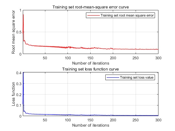
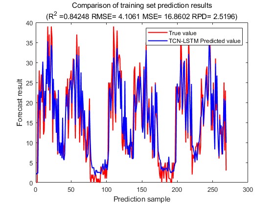
Figure 10: The change of loss. Figure 11: The predicted-actual value scatter plot.

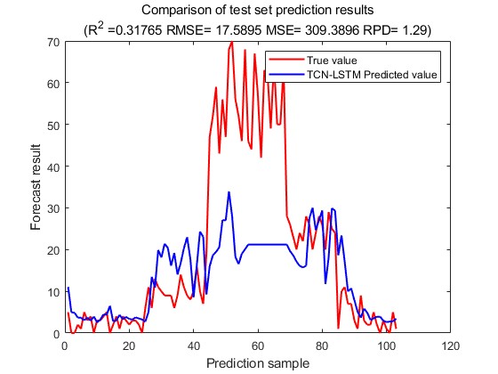
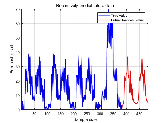
Figure 12: The predicted-actual value scatter plot. Figure 13: The prediction of the future traffic.

From the results of bike traffic prediction, it is clear that the model also shows good prediction on bike traffic prediction with R2 of 0.84 for the training set and R2 of 0.31 for the test set, which shows good results on the training set and slightly worse performance on the test set.

The final output is the result of the prediction of the truck traffic. The change in loss during training is shown in Fig. 14, the predicted-actual value scatter plot for the training set is shown in Fig. 15, and the predicted-actual value scatter plot for the test set is shown in Fig. 16, and the prediction of future traffic using the trained model is shown in Fig. 17.

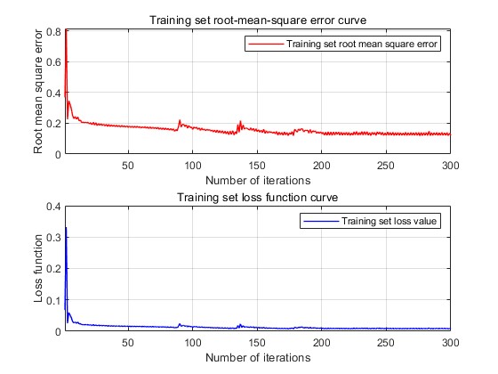
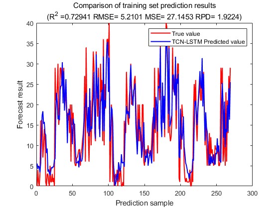
Figure 14: The change of loss. Figure 15: The predicted-actual value scatter plot.

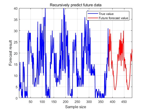
Figure 16: The predicted-actual value scatter plot. Figure 17: The prediction of the future traffic.

From the results of the truck traffic prediction, it can be seen that the R2 of the training set is 0.73 and the R2 of the test set is 0.50, which is a better prediction compared to the bicycle traffic and shows a good generalisation ability.

In order to verify the practical effect of the model, we conducted two sets of ablation experiments, using only the time-domain convolutional network algorithm and the long-short-term memory network algorithm to predict traffic flow, respectively, and quantitatively evaluated using the indicators of MAE, MSE, R^2, and RPD, and the results are shown in Table 2.

Table 2: Results of ablation experiments.

From the results of the ablation experiments, it can be seen that the TCN-LSTM hybrid model is the best, with a reduction of 0.11 in MAE compared to TCN, and TCN-LSTM is located between TCN and LSTM in MSE, and also the highest among the three in RPD, which indicates that the TCN-LSTM in this paper has the strongest predictive ability.

5. Conclusion

In this study, a hybrid model based on time-domain convolutional network (TCN) optimised long-short-term memory network (TCN-LSTM) is proposed to address the complex temporal characteristics of traffic flow prediction, and its effectiveness is verified in the tasks of automobile, bicycle, and truck traffic flow prediction through multiple sets of comparative experiments.

In the car traffic prediction task, the model demonstrates excellent convergence and generalisation ability. The loss function decreases steadily from the initial value of 0.8 to below 0.1 and tends to be stable during the training process, and the R² of the training set and the test set reaches 0.73 and 0.75, respectively, indicating that the model is not only able to fully learn the nonlinear features in the data, but also able to effectively overcome the overfitting problem. This result verifies the ability of TCN-LSTM to model the continuity and periodicity of automobile flow, and the synergy between its deep feature extraction module (TCN) and the sequence dynamic memory module (LSTM) makes the model capable of capturing the short-term fluctuations of vehicle aggregation in the road network as well as correlating the long-period patterns such as morning and evening peaks. For bicycle flow prediction, the model achieves a high R² value of 0.84 on the training set, but the R² drops to 0.31 on the test set, reflecting the fact that bicycle flow may be more stochastic and environmentally sensitive (e.g., external disturbances such as sudden changes in the weather and bicycle-sharing scheduling), resulting in a widening of the difference between the training data distribution and the test scenario. Nevertheless, the high accuracy of the training set demonstrates the model's ability to characterise complex local patterns, while the fluctuation of the test performance suggests the need to enhance the model's robustness by introducing external variables in the future. In truck traffic prediction, the R² of the model's training and test sets are 0.73 and 0.50, respectively.

The comparative analysis of TCN, LSTM and TCN-LSTM through ablation experiments further reveals the structural advantages of hybrid models in this study. The experimental data show that the prediction error (MAE) of TCN-LSTM is 0.11 lower than that of the single TCN model, and the reduction of the mean absolute error intuitively reflects the complementary gains of the gating mechanism and the convolutional features; its mean squared error (MSE) is in-between those of the TCN and the LSTM, which suggests that the hybrid model achieves a compromise optimisation in balancing the sensitivity of local outliers and the overall stability; and the relative prediction The relative prediction deviation (RPD) reaches the highest value of the three, which statistically confirms the high consistency between the TCN-LSTM prediction results and the distribution of true values.

The significance of this study lies in the fact that through the deep coupling of TCN and LSTM, a traffic flow prediction framework that takes into account both local feature capture and global state evolution is constructed, which provides a new idea for solving the problem of multimodal traffic flow prediction in intelligent transport systems.

References

[1]. Pandey, Ashutosh, and DeLiang Wang. "TCNN: Temporal convolutional neural network for real-time speech enhancement in the time domain." ICASSP 2019-2019 IEEE International Conference on Acoustics, Speech and Signal Processing (ICASSP). IEEE, 2019.
[2]. Hou, Changbo, et al. "Multisignal modulation classification using sliding window detection and complex convolutional network in frequency domain." IEEE Internet of Things Journal 9.19 (2022): 19438-19449.
[3]. Teixeira, F. L., et al. "Finite-difference time-domain methods." Nature Reviews Methods Primers 3.1 (2023): 75.
[4]. Bai, Ruxue, et al. "Fractional Fourier and time domain recurrence plot fusion combining convolutional neural network for bearing fault diagnosis under variable working conditions." Reliability Engineering & System Safety 232 (2023): 109076.
[5]. Monsalves, N., et al. "Application of Convolutional Neural Networks to time domain astrophysics. 2D image analysis of OGLE light curves." Astronomy & Astrophysics 691 (2024): A106.
[6]. Liang, Pengfei, et al. "Unsupervised fault diagnosis of wind turbine bearing via a deep residual deformable convolution network based on subdomain adaptation under time-varying speeds." Engineering Applications of Artificial Intelligence 118 (2023): 105656.
[7]. Hou, Xiaoqi, and Yong Gao. "Single-channel blind separation of co-frequency signals based on convolutional network." Digital Signal Processing 129 (2022): 103654.
[8]. Shaaban, Ahmed, et al. "RT-SCNNs: real-time spiking convolutional neural networks for a novel hand gesture recognition using time-domain mm-wave radar data." International Journal of Microwave and Wireless Technologies 16.5 (2024): 783-795.
[9]. Qiu, Haobo, et al. "A piecewise method for bearing remaining useful life estimation using temporal convolutional networks." Journal of Manufacturing Systems 68 (2023): 227-241.
[10]. Tsaih, Rua-Huan, and Chih Chun Hsu. "Artificial intelligence in smart tourism: A conceptual framework." (2018)..
Cite this article
Liu,Y. (2025). Traffic Flow Prediction Model Based on the Fusion of Timedomain Convolutional Network and Long- and Short-term Memory Network. Applied and Computational Engineering,144,59-68.
Data availability
The datasets used and/or analyzed during the current study will be available from the authors upon reasonable request.
Disclaimer/Publisher's Note
The statements, opinions and data contained in all publications are solely those of the individual author(s) and contributor(s) and not of EWA Publishing and/or the editor(s). EWA Publishing and/or the editor(s) disclaim responsibility for any injury to people or property resulting from any ideas, methods, instructions or products referred to in the content.
About volume
Volume title: Proceedings of the 3rd International Conference on Functional Materials and Civil Engineering
© 2024 by the author(s). Licensee EWA Publishing, Oxford, UK. This article is an open access article distributed under the terms and
conditions of the Creative Commons Attribution (CC BY) license. Authors who
publish this series agree to the following terms:
1. Authors retain copyright and grant the series right of first publication with the work simultaneously licensed under a Creative Commons
Attribution License that allows others to share the work with an acknowledgment of the work's authorship and initial publication in this
series.
2. Authors are able to enter into separate, additional contractual arrangements for the non-exclusive distribution of the series's published
version of the work (e.g., post it to an institutional repository or publish it in a book), with an acknowledgment of its initial
publication in this series.
3. Authors are permitted and encouraged to post their work online (e.g., in institutional repositories or on their website) prior to and
during the submission process, as it can lead to productive exchanges, as well as earlier and greater citation of published work (See
Open access policy for details).