1. Introduction

Coverage path planning is a fundamental problem in robotics, where the goal is to ensure that a robot covers all accessible areas of a given environment[1]. This problem has significant applications in various fields[2], including cleaning robots, agricultural robots, and search-and-rescue operations. In search-and-rescue scenarios, autonomous robots are often deployed to explore disaster-stricken areas, such as collapsed buildings or earthquake zones, to locate survivors and assess the environment. Efficient coverage path planning is critical in these scenarios[3], as it ensures that the robot can systematically search the area while minimizing the time and energy required. Traditional approaches to coverage path planning often struggle to balance exploration (covering new areas) and exploitation (minimizing travel distance)[4]. This paper proposes a novel algorithm that addresses these challenges by dynamically selecting target points and incorporating visibility constraints. The proposed method is particularly suited for search-and-rescue missions, where the environment may contain obstacles, uneven terrain, and areas of varying priority.

2. Method

The proposed algorithm consists of four main components: map representation, dynamic target selection, path planning, and coverage updates. Detailed description of each component is provided below.

2.1. Map Representation

The environment is modeled as a 2D grid map \( M \) of size R×C, where each cell \( M(i, j) \) is assigned one of the following values:

• 0: Passable and requires coverage (PC)

In a search-and-rescue scenario, this could represent open areas where survivors might be located. The robot must thoroughly search these areas to ensure no survivors are missed.

• 1: Impassable and requires coverage (IC)

This could represent areas blocked by debris or obstacles that cannot be traversed by the robot but may still contain survivors. The robot must attempt to cover these areas without physically entering them.

• 2: Passable but does not require coverage (PN)

This could represent safe, open areas that have already been cleared or are unlikely to contain survivors. The robot can traverse these areas but does not need to spend time searching them.

• 3: Impassable and does not require coverage (IN)

This could represent permanent obstacles, such as walls or large machinery, that are known to be inaccessible and do not require further inspection. These obstacles are considered visual obstructions, so the blocked areas will not be marked covered although they are within the robot’s range of sight.

An illustrative example of environment map representation is depicted in Figure 1.

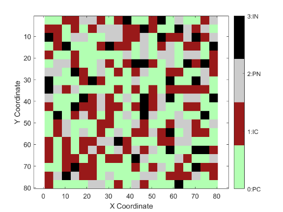
Figure 1: Environment map representation

Besides the environment map M, a Boolean coverage matrix C of the same size is initialized to track covered cells.

2.2. Coverage Update

The robot’s coverage area is updated using a visibility model that accounts for both visible and occluded regions within a \( d × d \) neighborhood of the robot’s current position \( (y, x) \) . For each cell in the neighborhood, the algorithm determines visibility by checking if the line of sight from the robot to the cell is blocked by impassable obstacles of type 3. This is achieved using Bresenham’s line algorithm[5] to generate a straight-line path between the robot’s position and the target cell. If any cell along this path is an obstacle of type 3, the target cell is considered occluded and is not marked as covered.

Specifically, the algorithm iterates over all cells within the \( d × d \) neighborhood. For each cell \( (i, j) \) , the following steps are performed:

• Visibility Check: A straight-line path is generated using Bresenham’s algorithm from \( (y, x) \) to \( (i, j) \) . Each cell along this path is checked for obstacles of type 3. If such an obstacle is encountered, the target cell is marked as occluded.

• Coverage Update: If the target cell \( (i, j) \) is not occluded and requires coverage (i.e., \( M(i, j) = 0 or M(i, j) = 1 \) ), it is marked as covered in the coverage matrix \( C \) .

This approach ensures that only cells with a clear line of sight are marked as covered, while occluded regions remain uncovered until the robot moves to a position where they become visible. The visibility model is critical for accurately simulating real-world scenarios where obstacles can block the robot’s sensors.

2.3. Dynamic Target Selection

To efficiently select target points, the algorithm first identifies all uncovered cells that require coverage, which constitute the set:

\( \lbrace (i,j) ∣(M(i,j) = 0 ∧C(i,j) = 0) ∨(M(i,j) = 2 ∧C(i,j) = 0)\rbrace \) (1)

From the set of uncovered cells, the algorithm selects a subset of candidate points for evaluation. This is done to reduce computational overhead and focus on the most promising targets. The candidate points are filtered based on their proximity to the robot's current position. Specifically, the algorithm selects the nearest 30 uncovered cells using the Manhattan distance[6] as the proximity metric.

The target selection process is guided by a scoring function that balances two objectives:

• Minimizing travel distance to the target.

• Maximizing the number of newly covered cells when the robot reaches the target.

The scoring function is defined as:

\( Score={w_{1}}\cdot \frac{1}{PathCost}+{w_{2}}\cdot \frac{Co{v_{new}}}{Co{v_{max}}}, \) (2)

where:

• \( {w_{1}}=a+(1-a)\cdot {R_{c}} \) is the weight for travel distance, in which \( {R_{c}} \) , or Coverage Ratio is calculated as:

\( {R_{c}}=\frac{\sum _{(i,j)}I((M(i,j)=0∨M(i,j)=1)∧C(i,j)=1)}{\sum _{(i,j)}I(M(i,j)=0∨M(i,j)=1)}, \) (3)

where:

– \( C(i,j) \) is the coverage matrix.

– \( M(i,j) \) is the map matrix.

– \( I(·) \) is the indicator function.

• \( {w_{2}}=1-{w_{1}} \) is the weight for coverage area.

• \( a \) is a user-defined parameter that controls the trade-off between exploration and exploitation.

• Path Cost represents the travel distance from the robot’s current position to the target. It is computed using the A* algorithm[7], which finds the shortest path while avoiding obstacles. The path cost is given by:

\( PathCost=\sum _{k=1}^{n-1}|{p_{k+1}}-{p_{k}}| \) (4)

where \( {p_{k}} \) is the k-th point on the path, and \( |\cdot | \) denotes the Euclidean distance between two points.

• \( Co{v_{new}} \) is the number of previously uncovered cells that become visible when the robot reaches the target. It is calculated as:

\( Co{v_{new}}=\sum _{(i,j)∈Visible Cells}I(C(i,j)=0∧(M(i,j)=0∨M(i,j)=1)), \) (5)

where \( Visible Cells \) are the cells within the robot’s visibility range \( d × d \) neighborhood.

• \( Co{v_{max}} \) is the maximum possible number of new cells that can be covered when the robot reaches the target. It is defined as:

\( Co{v_{max}}=\sum _{(i,j)∈Visible Cells}I(M(i,j)=0∨M(i,j)=1). \) (6)

This represents the total number of cells within the robot’s visibility range that require coverage.

The weight \( {w_{1}} \) in the scoring function dynamically adjusts the balance between exploration and exploitation. When the coverage ratio is low, \( {w_{1}} \) is dominated by \( a \) , and the algorithm prioritizes exploration (covering new areas). When the coverage ratio is high, \( {w_{1}} \) approaches 1, and the algorithm prioritizes minimizing travel distance.

2.4. Path Planning

Once a target is selected, the A* algorithm is used to compute the optimal path from the robot’s current position to the target. The A* algorithm employs the Euclidean distance as the heuristic function to ensure efficient path-finding. If no valid path exists, the target is discarded, and the algorithm selects the next best target.

2.5. Main Loop

The algorithm iterates until the coverage ratio exceeds a predefined threshold (e.g., 95%) or no further uncovered areas are available. In each iteration:

• The robot moves along the computed path to the target.

• The coverage matrix \( C \) is updated based on the robot’s new position.

2.6. Termination

The algorithm terminates when:

• The coverage ratio exceeds the threshold.

• No further uncovered areas are reachable.

• The robot cannot find a valid path to any target.

A simplified program flow chart is shown in Figure 2.

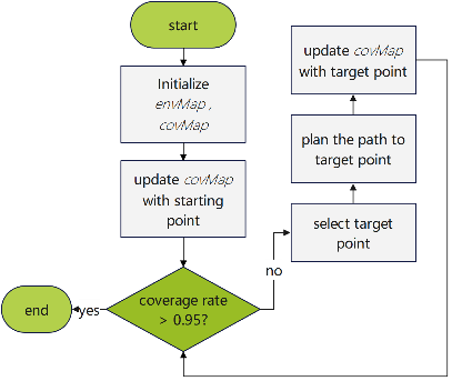
Figure 2: Program flowchart

3. Experiments

To evaluate the performance of the proposed algorithm, a series of experiments were conducted to investigate the relationship between the total travel distance and two key factors: the parameter \( a \) , and map size. The experiments were designed to analyze how these factors influence the algorithm's efficiency in terms of coverage and path optimization.

3.1. Experimental Setup

The experiments were conducted on synthetic grid maps with the following configurations:

• Visibility range: 10 × 10 neighborhood.

• Coverage ratio threshold: 95%.

For each combination of map size and a value, the algorithm was run 10 times, and the average total travel distance was recorded.

3.2. Relationship Between Total Distance and \( a \)

Figure 3 shows the relationship between the total travel distance and the parameter a for different map sizes. The results indicate that: For small maps (30 × 30 to 50 × 50), the value of a has little influence to the total distance. At \( a=0 \) , the total distance is relatively small, and at \( a=1 \) , the total distance tends to be larger. However, for medium-sized maps (60 × 60 to 90 × 90), the total distance exhibits significant fluctuation with varying values of \( a \) . At \( a=0 \) , the total distance is relatively large, and at \( a=1 \) , the total distance tends to be smaller. The optimal value for \( a \) appears to be 0.7. Finally, for big maps (larger than 90 × 90), the total distance decreases as \( a \) increases.

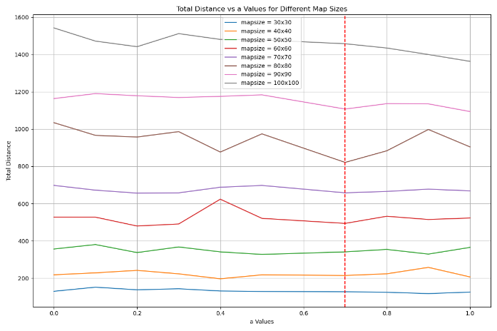
Figure 3: Total travel distance- \( a \) for different map sizes.

The observed behavior can be explained as follows: In small maps, the robot can efficiently cover the entire area without being significantly affected by the value of \( a \) . The limited size reduces the impact of the exploration-exploitation trade-off, resulting in stable total distances across different values of \( a \) . However, in larger maps, the robot must navigate a much larger area, making the trade-off between exploration and exploitation more critical. When \( a \) is low, the robot prioritizes exploration, which may leave some areas insufficiently explored, leading to longer travel distances. When \( a \) is high, the robot prioritizes making smaller steps, and therefore minimizing total distance.

3.3. Relationship Between Total Distance and Map Size

Figure 4 illustrates the relationship between the total travel distance and map size for different values of a and obstacle densities. The results demonstrate that: as the map size increases, the total travel distance increases at a growing pace due to the increased complexity of path planning. This trend is consistence among different values of \( a \) , indicating that the trade-off between exploration and exploitation has a similar effect across all map sizes.

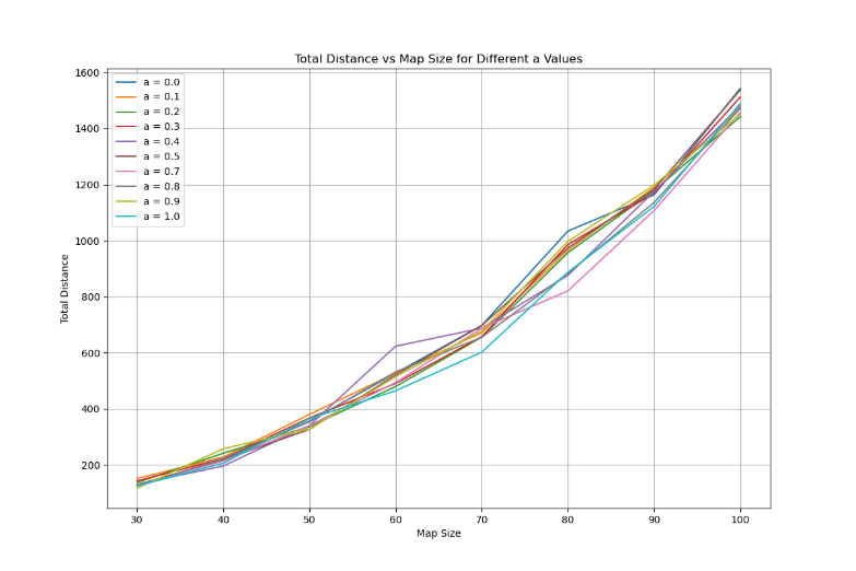
Figure 4: Total travel distance- map size for different values of \( a \) .

These findings provide valuable insights for optimizing the performance of the proposed algorithm in various real-world scenarios.

4. Conclusions

This paper presents a novel coverage path planning algorithm that dynamically selects target points based on a weighted scoring function, incorporating visibility constraints to ensure efficient coverage in grid-based environments. The algorithm effectively balances exploration and exploitation through a dynamic weight adjustment mechanism, leveraging the A* path planning algorithm to optimize travel distance. Experimental results demonstrate that the proposed method significantly reduces travel distance while maximizing coverage across various map sizes and configurations. Depending on relative map sizes, the value of \( a \) can be adjusted according to the following rules: When the map size is less than 10 times the detection range, the value of \( a \) is not significant; when the map size is between 10 and 25 times the detection range, \( a \) is best set at 0.7; when the map size is greater than 25 times the detection range, a is best set at 1.

Future research will concentrate on the integration of machine learning techniques for the real-time adjustment of parameter \( a \) in response to environmental feedback. Moreover, this study will undertake field experiments in actual search-and-rescue scenarios to ascertain the algorithm’s performance and adaptability.

References

[1]. Murphy, R., Tadokoro, S., Nardi, D., Jacoff, A., Fiorini, P., Choset, H., & Erkmen, A. (2008). Search and rescue robotics. In B. Siciliano & O. Khatib (Eds.), Springer handbook of robotics(pp. 1151-1173). Springer. https://doi.org/10.1007/978-3-540-30301-5_51
[2]. Overmars, M. H., & van der Stappen, A. F. (1997). Motion planning in the plane. In M. de Berg, M. van Kreveld, M. Overmars, & O. Schwarzkopf (Eds.), Computational geometry: Algorithms and applications(2nd ed., pp. 225-253). Springer-Verlag.
[3]. Choset, H. (2001). Coverage for robotics—A survey of recent results. Annals of Mathematics and Artificial Intelligence, 31(1-4), 113–126. https://doi.org/10.1023/A:1016639210959
[4]. Hart, P. E., Nilsson, N. J., & Raphael, B. (1968). A formal basis for the heuristic determination of minimum cost paths. IEEE Transactions on Systems Science and Cybernetics, 4(2), 100-107. https://doi.org/10.1109/TSSC.1968.300136
[5]. Bresenham, J. E. (1965). Algorithm for computer control of a digital plotter. IBM Systems Journal, 4(1), 25–30. https://doi.org/10.1147/sj.41.0025
[6]. Deza, E., & Deza, M. M. (2009). Encyclopedia of Distances. Springer. Minkowski, H. (1910). Geometrie der Zahlen. Teubner.
[7]. Koenig, S., & Likhachev, M. (2002). D* Lite. In Proceedings of the AAAI Conference on Artificial Intelligence (pp. 476–483). AAAI Press.
Cite this article
Ding,Z. (2025). Coverage Path Planning with Dynamic Target Selection for Search and Rescue. Applied and Computational Engineering,145,7-13.
Data availability
The datasets used and/or analyzed during the current study will be available from the authors upon reasonable request.
Disclaimer/Publisher's Note
The statements, opinions and data contained in all publications are solely those of the individual author(s) and contributor(s) and not of EWA Publishing and/or the editor(s). EWA Publishing and/or the editor(s) disclaim responsibility for any injury to people or property resulting from any ideas, methods, instructions or products referred to in the content.
About volume
Volume title: Proceedings of the 3rd International Conference on Software Engineering and Machine Learning
© 2024 by the author(s). Licensee EWA Publishing, Oxford, UK. This article is an open access article distributed under the terms and
conditions of the Creative Commons Attribution (CC BY) license. Authors who
publish this series agree to the following terms:
1. Authors retain copyright and grant the series right of first publication with the work simultaneously licensed under a Creative Commons
Attribution License that allows others to share the work with an acknowledgment of the work's authorship and initial publication in this
series.
2. Authors are able to enter into separate, additional contractual arrangements for the non-exclusive distribution of the series's published
version of the work (e.g., post it to an institutional repository or publish it in a book), with an acknowledgment of its initial
publication in this series.
3. Authors are permitted and encouraged to post their work online (e.g., in institutional repositories or on their website) prior to and
during the submission process, as it can lead to productive exchanges, as well as earlier and greater citation of published work (See
Open access policy for details).