1. Introduction

Stock price prediction is crucial for investment decisions, risk reduction, and market efficiency. Traditional econometric models (e.g., ARIMA, GARCH) have limitations due to simplified assumptions (Kumar et al.[1]; Petrica et al.[2]). Recent advances in Machine Learning (ML), particularly Random Forest (RF), show superior performance in nonlinear modeling and feature extraction (Khedr et al.[3]; Mintarya et al.[4]; Khaidem et al.[6]). However, RF's performance relies heavily on hyperparameter tuning, involving trade-offs between accuracy, efficiency, and generalization (Probst et al.[7]). Traditional optimization methods (e.g., Random Search, Grid Search) are inefficient and often fail to identify optimal solutions (Yang et al.[8]; Bischl et al.[9]).

This study employs Particle Swarm Optimization (PSO) for hyperparameter optimization due to its faster convergence, fewer parameter settings, and ability to avoid local optima in high-dimensional problems (Li et al.[10]; Juneja et al.[11]; Reif et al.[12]). PSO's key parameters include inertia weight (w), learning factors (c1 and c2), swarm size (n), and number of iterations, with values set based on Syi et al.[13]. The study also incorporates technical indicators (e.g., EMA, RSI) and market activity features (e.g., trading volume) to enhance trend capture, considering the market's dynamic and uncertain nature (Tsay et al.[14]). The hybrid PSO-RF model aims to improve prediction accuracy and efficiency.

The paper is structured as follows: Section 2 covers data processing and statistics; Section 3 focuses on time series analysis, including the Augmented Dickey-Fuller (ADF) test (Mushtaq et al.[15]), white noise test, and correlation test; Section 4 details the methodology and model construction; Section 5 presents the model prediction results and performance comparisons with benchmarks (PSO-SVM, Grid-RF, GA-RF); Section 6 concludes the study and proposes further research prospects.

2. Data

2.1. Data Source

The study utilizes data from Tushare, a professional financial data platform for quantitative research, covering stocks, funds, and futures. The research focuses on stock 300056.SZ (Zhongchuang Environmental Protection) from February 13, 2014, to December 30, 2022. The dataset includes nine variables: Open, High, Low, Close, Change, Pct_chg, Vol, and Amount, comprising 1924 data points.

2.2. Feature Construction

To build an effective prediction model, this paper selects the following features as model inputs. These features reflect the operating status of the stock market from multiple perspectives and enhance the model's ability to capture market trends. The following are the selected features and their definitions. (Table 1).

Table 1: Feature Selection

Change represent the difference between the current day's closing price and the previous trading day's closing price, capturing the absolute change in stock price. Meanwhile, Pct_chg denotes the percentage change between the current day's closing price and the previous trading day's closing price, quantifying the relative change in stock price.

2.3. Data Processing

2.3.1. Missing Value Handling

Due to the closure of the stock market on weekends and holidays, the original data contains missing values. This paper employs linear interpolation to fill in the missing values. By calculating the linear relationship between the preceding and succeeding valid data points, the missing values are estimated while retaining the time series characteristics of the data, providing a reliable basis for subsequent analysis.

2.3.2. Data Normalization

To eliminate the differences in scales and ranges of different features, this paper adopts the Min-Max normalization method to scale each feature's data into the [0, 1] interval, thereby enhancing the model's training effectiveness and prediction accuracy. The Min-Max normalization formula is as follows: (Equation 1)

\( x\_scaled=\frac{x-min⁡(x)}{max{(x)}-min⁡(x)} \) (1)

where x is a value in the original data, min(x) and max(x) are the minimum and maximum values in the dataset, respectively.

3. Time Series Analysis

3.1. Initial Data Time Series Plot

After completing data preprocessing, this paper conducts a time series analysis to understand the data characteristics better and lay the foundation for subsequent model construction. First, the time series plot of the stock closing price is drawn. (Figure 1).

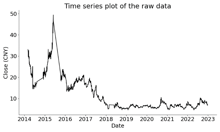
Figure 1: Time series plot of the raw data

3.2. Stationarity Test

3.2.1. ADF Test

The ADF test assesses stationarity by testing the null hypothesis of a unit root (non-stationarity) against the alternative of stationarity. A p-value below 0.05 rejects the null hypothesis, indicating stationarity. For the raw data, the ADF test yields a p-value of 0.093, failing to reject the null hypothesis and confirming non-stationarity.To achieve stationarity, first-order differencing is applied, and the test is repeated. The differenced time series exhibits more uniform fluctuations. (Figure 2). The ADF test results for the differenced data show a p-value significantly below 0.05, rejecting the null hypothesis and confirming stationarity.

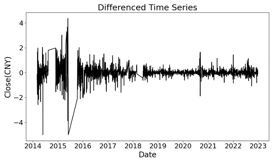
Figure 2: Time series plot of data after first-order differencing

3.2.2. Lag Order Selection

The selection of lag order is crucial for the accuracy of the time series model. This paper examines the autocorrelation function (ACF) plot and partial autocorrelation function (PACF) plot, revealing periodicity in the sequence. (Figure 3, Figure 4). Further, by combining the Akaike Information Criterion (AIC) and Bayesian Information Criterion (BIC), the optimal lag order is determined to be 7.

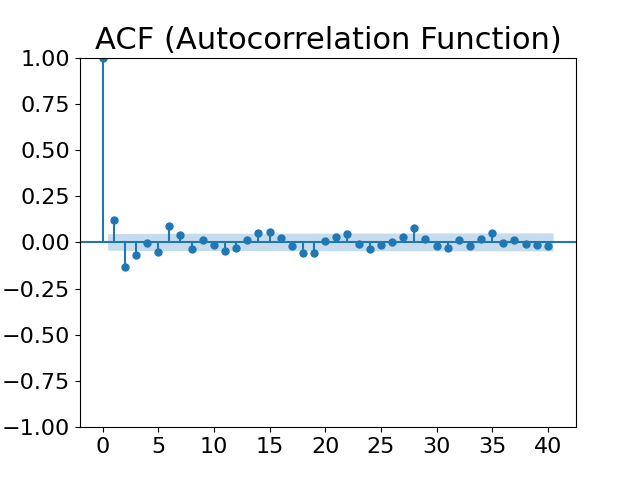
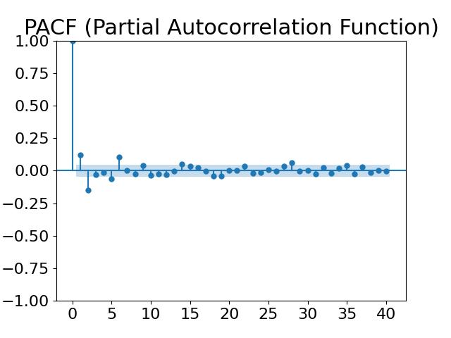
Figure 3: ACF plot Figure 4: PACF plot

3.2.3. White Noise Test (Pure Randomness Test)

The white noise test is crucial for assessing time series predictability. A non-white noise sequence contains structured information suitable for modeling. This study applies the Ljung-Box Q test to the original and first-order differenced time series. (Table 3). With p-values significantly below 0.05, the null hypothesis is rejected, confirming significant autocorrelation and non-white noise characteristics. This structured information provides a foundation for subsequent model development.

Table 3: Ljung-Box Q test results of original data

3.3. Correlation Analysis

The study examines the linear relationships between each feature and the closing price via correlation analysis to inform feature selection and model construction(Figure 5). The results indicate strong positive correlations between Open, High, and Low prices and the closing price (coefficients > 0.85). EMA and RSI also show positive correlations (coefficients of 0.82 and 0.44, respectively). These significant linear relationships suggest that these features can serve as input variables for the Random Forest model to predict stock closing prices.

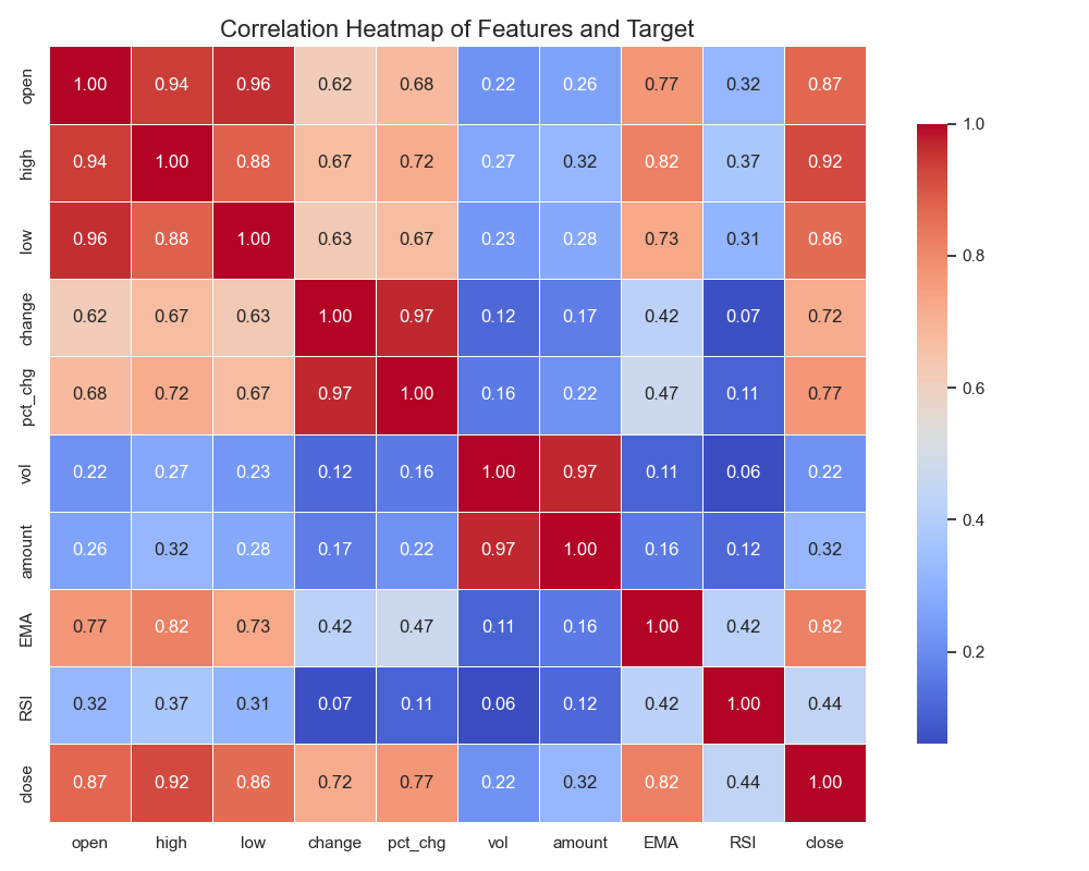
Figure 5: Correlation coefficient heatmap

4. Methodology

4.1. Random Forest (RF)

Random Forest (RF), proposed by Leo Breiman, is an ensemble learning algorithm that constructs multiple decision trees to enhance generalization. It uses Bootstrap sampling (Efron et al.[16]) to draw subsamples from the dataset, training each tree independently. During node splitting, trees select optimal split points from a random subset of features (Hasan et al.[17]), reducing overfitting and enabling high-dimensional data handling. The final prediction is aggregated via majority voting (classification) or averaging (regression), improving stability and accuracy. (Figure 6).

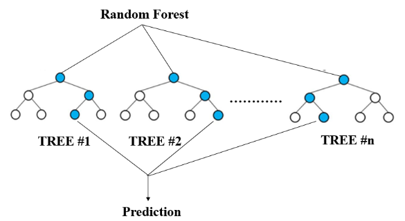
Figure 6: Random Forest (RF) illustration

4.2. Particle Swarm Optimization (PSO)

Particle Swarm Optimization (PSO) is an optimization algorithm that simulates the foraging behavior of bird flocks, achieving global optimization through particle collaboration. Each particle represents a potential solution and has position and velocity attributes. At the initial stage, the velocity vi​(0) and position xi​(0) of each particle are randomly initialized, and the individual best solution pbesti​ and global best solution gbest are recorded. The velocity and position of the particles are updated according to the following formulas:

Velocity update formula:(Equation 2)

\( {v_{i}}(t+1)=w·{v_{i}}(t)+{c_{1}}·{r_{1}}·({pbest_{i}}-{x_{i}}(t))+{c_{2}}·{r_{2}}·(gbest-{x_{i}}(t)) \) (2)

Position update formula:(Equation 3)

\( {x_{i}}(t+1)={x_{i}}(t)+{v_{i}}(t+1) \) (3)

where w is the inertia weight, c1​ and c2​ are learning factors, and r1​ and r2​ are random numbers that control the particle's dependence on individual and swarm experience. The algorithm iterates until a predefined termination condition is met, such as reaching the maximum number of iterations or the change in the solution being less than a set threshold.

5. Results

5.1. PSO-RF Prediction Results

PSO-RF model’s parameter, search range, and optimized parameter settings are as follows. (Table 4).

Table 4: PSO-RF model parameter search range and optimal parameter settings

To initially demonstrate the prediction performance of the PSO-RF model on stock prices, a prediction line chart is drawn. (Figure 7). Despite the impact of fitting for data on weekends and holidays when the stock market is closed, the PSO-RF model shows high accuracy in stock price prediction overall.

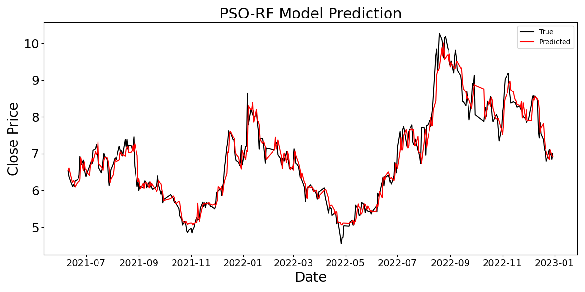
Figure 7: PSO-RF model prediction diagram

5.2. Feature Importance Analysis of RF

By summing the importance of features within the same category (e.g., Open, High, EMA, etc.), the total feature importance for each category is calculated. (Figure 8(a)). The analysis reveals that RSI has the greatest impact on model predictions, accounting for approximately 68.13% of the importance. This indicates a strong association between RSI and stock price changes. EMA, as a smoothing technical indicator, also significantly influences the prediction results. Other features, such as Amount and Vol, contribute to the model's predictions, while Open and High have relatively smaller impacts. From a temporal perspective, the importance of features at different lag days is shown. (Figure 8(b)). The results indicate that features from Day 1 (the previous day) have the greatest impact on model predictions, accounting for 67.58% of the importance. The importance of features decreases gradually with increasing lag days. This suggests that stock price predictions strongly depend on short-term features, especially those from the previous day, reflecting the inertia effect in stock price movements.

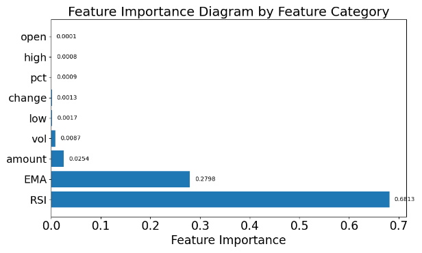
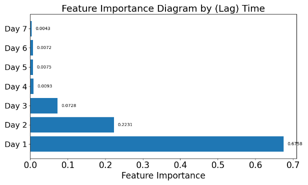
Figure 8(a): Importance by category Figure 8(b): Importance by (Lag) Time

5.3. Model Comparison

To comprehensively evaluate the performance of the PSO-RF model, this paper compares it with three benchmark models: PSO-SVM, Grid-RF, and GA-RF. The parameter settings for each model are shown. (Table 5).

Table 5: Parameter settings for Benchmarks

The evaluation metrics include MAE, MSE, RMSE, and R², results are as follows. (Table 6).

Table 6: Evaluation metrics results for each model

To more intuitively compare the prediction performance of the four models, prediction time series plots and Mean Relative Error (MRE) plots are drawn for all models. (Figure 9, Figure 10). The MRE during model training is defined as:(Equation 4)

\( MRE=\frac{1}{N}\sum _{i=1}^{N}|\frac{{Y_{i}}-{X_{i}}}{{Y_{i}}}| \) (4)

where Xi​ is the predicted value, Yi​ is the actual value, and N is the total number of samples. The mean relative error is calculated using a 7-day lag as a sliding window to assess the prediction accuracy over a short time range.

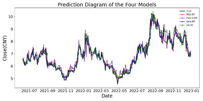
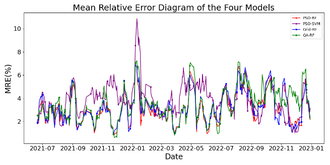
Figure 9: Prediction diagram Figure 10: Mean relative error diagram

Time series plots indicate that the PSO-RF model outperforms other models, showing smoother performance and a higher fit with actual values, especially during volatility. It also exhibits lower MRE values and smaller error fluctuations, demonstrating superior accuracy and stability. Comparative analysis confirms its superior ability to capture market trends and fluctuations, particularly during major changes, making it the best-performing model in this experiment. The Diebold-Mariano (DM) test validates the PSO-RF model's superiority by assessing prediction accuracy differences. Results show significant differences in prediction accuracy compared to benchmarks (P-value < 0.05), confirming its superiority (Table 6).

Table 6: DM test results of PSO-RF with other models

6. Discussion

The PSO-RF model exhibits high accuracy and stability in stock price prediction, with R² = 0.943, MAE = 0.030, RMSE = 0.041, and MSE = 1.732×10⁻³. The Diebold-Mariano test confirms its superiority over benchmarks (PSO-SVM, Grid-RF, GA-RF) with P-values of less than 0.05. PSO's global search capability enhances hyperparameter optimization, overcoming grid search limitations and yielding lower RMSE (0.041 vs. 0.042 for Grid-RF). PSO also converges faster than GA (5 iterations vs. 10) and achieves higher R² (0.943 vs. 0.927 for GA-RF). The choice of RF over SVM is significant, as RF's ability to handle high-dimensional data and avoid overfitting provides an advantage over SVM, which is more sensitive to kernel selection and computational complexity (MAE: 0.030 for PSO-RF vs. 0.037 for PSO-SVM). The synergistic effect between PSO and RF enhances performance, with PSO overcoming RF's local optimum limitations and RF providing feedback to PSO. Feature importance analysis highlights RSI (68.1%) and the lagged "Day 1" feature (67.6%) as critical for capturing short-term market fluctuations.

7. Conclusion

This study constructs a hybrid PSO-RF model for stock price prediction using historical data of Zhongchuang Environmental Protection (300056.SZ) from Tushare. The model incorporates features such as opening price, EMA, and RSI. Stationarity and autocorrelation are confirmed via ADF and Ljung-Box Q tests. PSO optimizes RF hyperparameters, achieving strong performance. The DM-test shows superiority over benchmarks (PSO-SVM, Grid-RF, GA-RF), with feature importance analysis highlighting RSI and Day 1 features. Future work can focus on expanding feature selection, improving optimization algorithms, validating model universality, and integrating deep learning techniques (e.g., LSTM, Transformer) with PSO to enhance stock market analysis.

References

[1]. I. Kumar, K. Dogra, C. Utreja, P. Yadav, "A comparative study of supervised machine learning algorithms for stock market trend prediction," 2018 Second International Conference on Inventive Communication and Computational Technologies (ICICCT), IEEE, 2018, pp. 1003-1007.DOI: 10.1109/ICICCT.2018.8376099
[2]. A.-C. Petrică, S. Stancu, A.J.T. Tindeche, "Limitation of ARIMA models in financial and monetary economics," Annals of Economics, 23(4) (2016).DOI: 10.1515/aoe-2016-0025
[3]. A.M. Khedr, I. Arif, M. El‐Bannany, S.M. Alhashmi, M.J.I.S.i.A. Sreedharan, "Cryptocurrency price prediction using traditional statistical and machine‐learning techniques: A survey," Finance, Management, 28(1) (2021) 3-34.DOI: 10.1002/fima.12345
[4]. L.N. Mintarya, J.N. Halim, C. Angie, S. Achmad, A.J.P.C.S. Kurniawan, "Machine learning approaches in stock market prediction: A systematic literature review," Journal of Physics: Conference Series, 216 (2023) 96-102.DOI: 10.1088/1742-6596/216/1/012012
[5]. S.J.J.J.o.I.M. Rigatti, "Random forest," Journal of Investment Management, 47(1) (2017) 31-39.DOI: 10.2139/ssrn.2974937
[6]. L. Khaidem, S. Saha, S.R.J.a.p.a. Dey, "Predicting the direction of stock market prices using random forest," Journal of Financial Engineering, (2016).DOI: 10.1142/S2346001916500035
[7]. P. Probst, M.N. Wright, A.L.J.W.I.R.d.m. Boulesteix, "Hyperparameters and tuning strategies for random forest," Wiley Interdisciplinary Reviews: Data Mining and Knowledge Discovery, 9(3) (2019) e1301.DOI: 10.1002/widm.1301
[8]. L. Yang, A.J.N. Shami, "On hyperparameter optimization of machine learning algorithms: Theory and practice," IEEE Access, 415 (2020) 295-316.DOI: 10.1109/ACCESS.2020.3012345
[9]. B. Bischl, M. Binder, M. Lang, T. Pielok, J. Richter, S. Coors, J. Thomas, T. Ullmann, M. Becker, A.L.J.W.I.R.D.M. Boulesteix, "Hyperparameter optimization: Foundations, algorithms, best practices, and open challenges," Wiley Interdisciplinary Reviews: Data Mining and Knowledge Discovery, 13(2) (2023) e1484.DOI: 10.1002/widm.1484
[10]. Y. Li, Y.J.a.p.a. Zhang, "Hyper-parameter estimation method with particle swarm optimization," IEEE Transactions on Cybernetics, (2020).DOI: 10.1109/TCYB.2020.3012345
[11]. M. Juneja, S. Nagar, "Particle swarm optimization algorithm and its parameters: A review," 2016 International Conference on Control, Computing, Communication and Materials (ICCCCM), IEEE, 2016, pp. 1-5.DOI: 10.1109/ICCCCM.2016.7856789
[12]. D.M. Reif, A.A. Motsinger, B.A. McKinney, J.E. Crowe, J.H. Moore, "Feature selection using a random forests classifier for the integrated analysis of multiple data types," IEEE Symposium on Computational Intelligence and Bioinformatics and Computational Biology, IEEE, 2006, pp. 1-8.DOI: 10.1109/CIBCB.2006.1673123
[13]. Y. Shi, R.C. Eberhart, "Parameter selection in particle swarm optimization," Evolutionary Programming VII: 7th International Conference, EP98 San Diego, California, USA, March 25–27, 1998 Proceedings, 7, Springer, 1998, pp. 591-600.DOI: 10.1007/BFb0040819
[14]. R.S. Tsay, Multivariate time series analysis: with R and financial applications, John Wiley & Sons, 2013.DOI: 10.1002/9781118617908
[15]. R. Mushtaq, "Augmented dickey fuller test," Journal of Statistical Theory and Applications, (2011).DOI: 10.2991/jsta.2011.10.1.1
[16]. B. Efron, R.J.B. Tibshirani, "The bootstrap method for assessing statistical accuracy," Statistical Science, 12(17) (1985) 1-35.DOI: 10.1214/ss/1177005852
[17]. M.A.M. Hasan, M. Nasser, S. Ahmad, K.I.J.J.o.i.s. Molla, "Feature selection for intrusion detection using random forest," Journal of Information Security, 7(3) (2016) 129-140.DOI: 10.4236/jis.2016.73012
[18]. H. Chen, Q. Wan, Y.J.E. Wang, "Refined Diebold-Mariano test methods for the evaluation of wind power forecasting models," Energy Conversion and Management, 7(7) (2014) 4185-4198.DOI: 10.1016/j.enconman.2014.07.028
Cite this article
Kong,J. (2025). A Novel Hybrid Model for Accurate Stock Market Forecasting Based on PSO and RF. Applied and Computational Engineering,146,23-32.
Data availability
The datasets used and/or analyzed during the current study will be available from the authors upon reasonable request.
Disclaimer/Publisher's Note
The statements, opinions and data contained in all publications are solely those of the individual author(s) and contributor(s) and not of EWA Publishing and/or the editor(s). EWA Publishing and/or the editor(s) disclaim responsibility for any injury to people or property resulting from any ideas, methods, instructions or products referred to in the content.
About volume
Volume title: Proceedings of SEML 2025 Symposium: Machine Learning Theory and Applications
© 2024 by the author(s). Licensee EWA Publishing, Oxford, UK. This article is an open access article distributed under the terms and
conditions of the Creative Commons Attribution (CC BY) license. Authors who
publish this series agree to the following terms:
1. Authors retain copyright and grant the series right of first publication with the work simultaneously licensed under a Creative Commons
Attribution License that allows others to share the work with an acknowledgment of the work's authorship and initial publication in this
series.
2. Authors are able to enter into separate, additional contractual arrangements for the non-exclusive distribution of the series's published
version of the work (e.g., post it to an institutional repository or publish it in a book), with an acknowledgment of its initial
publication in this series.
3. Authors are permitted and encouraged to post their work online (e.g., in institutional repositories or on their website) prior to and
during the submission process, as it can lead to productive exchanges, as well as earlier and greater citation of published work (See
Open access policy for details).