1. Introduction

With the rapid development of multimedia technology and Internet equipment, social networks are filled with a large number of images, audio, video and other information. Among them, image, as one of the important data forms in the big data era, is the main way for human beings to exchange information with the outside world and contains rich content. How to filter out irrelevant and useless information from these huge images, filter out important information, and further apply it to practical problems is a hot issue in the current image field. Image recognition has always been a hot research issue in the field of computer vision, aiming at training models to automatically predict the categories of objects contained in a given image. Image recognition technology simulates the visual perception and understanding process of human brain through computer technology, modern information processing and other technical means, extracts image features according to some image processing methods, and takes the extracted features as the basis for final classification and recognition. In recent years, with the rapid development of machine learning and computer vision, image classification and recognition has been widely used in various fields, such as face recognition technology in the field of security, vehicle recognition technology in the field, of transportation and aviation remote sensing in the field of aeraspace and so on.

Early image recognition methods mostly rely on manual features, and their basic processes include image preprocessing, image feature extraction and classifier design. The selection and design of manual features is the key of traditional image recognition methods. Commonly used manual features include color, texture, shape, gradient, etc., such as hog, LBP, sift, surf, siltp, etc. Although this traditional method is effective for some simple images, its accuracy cannot meet the actual application requirements for other more complex or slightly different images. In recent years, thanks to the development of deep learning, image recognition algorithms based on convolutional neural network (CNN) have gradually become the mainstream of research, greatly improving the accuracy and speed of recognition. The structure of the convolutional neural network typically consists of an input layer, a convolution layer, a regrouping layer, a complete connecting layer and an exit layer.. Convolutional neural network adopts the method of local connectivity and weight distribution: first, it reduces the number of weights in order to facilitate the calculation of the network easily; second, it also lesssens the complexity of the model and the potential for overflow, that is, it directly uses the image as the input of the network, and avoids the complexity increase caused by the function extraction process within the traditional recognition algorithm.. In the processing of two-dimensional images, convolutional neural network has great advantages. It can extract the features of images by itself. Especially in the face of identifying the invariance of deformation such as displacement and scale, convolutional neural network provides good robustness and efficiency of computation. In the field of image classification, the development of CNN has greatly improved the classification effect of image classification.

Focusing on traditional and deep learning based image recognition algorithms, in this paper, we first introduce the representative book recognition algorithms and analyze their advantages and disadvantages. In addition, common image recognition data sets and evaluation indexes are introduced, and the results of representative methods are compared quantitatively. Finally, we summarize the existing research problems in the image reconnaissance field and discuss the possible future development of this field.

2. Traditional image classification algorithm

2.1. K-Nearest neighbor

KNN is first developed by Evenlyn Fix and Joseph Hodges[1] in 1951 and later expanded by Thomas Cover[2]. The design idea of KNN is birds of a feather flock together. A sample alse belongs to this category if the majority of some most similar samples in the feature space belong to the same category.

In general, KNN algorithm include prepare data and pretreatment data, calculate the distance between test point and all remaining sample points, sort each distance in order and select the k points which is the nearest distance, compare the K points’ categories and then classified the test point in the category with the largest proportion among the K points these four steps.

The advantages of KNN is that: easy to implement and intuitive to understand, allow learning about nonlinear decisional limits when used for classifying and regressing, is able to offer an extremely flexible decision limit which adjusts the value of K, does not require training time to classify and regression[3]. Certainly, there are some disadvantages to this algorithm. First, it does not work well with large datasets. Second, because it becomes challenging for the algorithm to calculate the distance in each dimension with large numbers, does not perform well with high dimensions. Third, it needs feature scaling before applying KNN algorithm to any datasets because it may generate wrong predictions if we don’t do so[4].

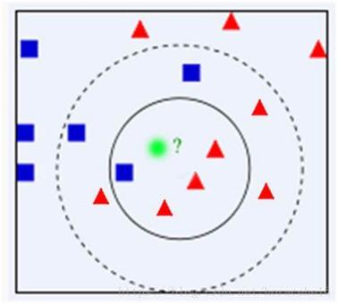
Figure 1. KNN.

2.2. Naive bays model

The definition of Naive Bays in machine learning is a probabilistic model in the supervised learning is a probabilistic model in the supervised learning genre that is employed in a variety of application scenarios, primarily classification, it presumes that each component of the model is independent of the others, or in other words, that changing one variable has no impact on the other variables[5]. This algorithm solves the ‘backward probability’ problem in probability theory.

Naive Bays Algorithm has roughly three steps: data processing, training and testing. In the data processing stage, it will extract feature attributes, classify and label data and then form the datasets. In training stage, the happening frequency of each group in the training samples and the conditional likelihood of each feature attribute segmentation for each class are calculated. Finally, it will training in the test step[6].

There are some advantages of naive bays model. First, this algorithm works speedily and can save plenty of time up. Second, it is suitable for working multi-class projection problems out. Third, if its supposition of features' independence holds true, it can operate better than other models and depends on much less training data. Last, it is better suitable for unconditional input variables than numeric variables[7]. This algorithm also has some disadvantages: The suppose of naive bays seldom happening in actual life. This situation leads to the fact that the applicability of this algorithm in real life is not good. Data shortage is another issue. You must calculate a likelihood value using a frequent its technique for each possible value of a feature. Probabilities may shift towards 0 or 1, which would produce poorer outcomes and numerical instability. If you smooth your probabilities in this situation or apply a prior to your data, you may claim that the resulting classifier is no longer naive[8].

2.3. Decision tree

A technique called decision tree classification uses a number of training samples without any kind of order or rules to infer classification rules for a decision tree representation form. It compares attribute values at the internal nodes of the decision tree using the top-down approach and evaluates the downward branch from the node based on various attribute values in order to arrive at the decision at the node of the decision tree.[9].

The generation of decision tree is divided into node splitting, determination of decision boundary, repeat and stop growth this three steps. Node splitting is means when a node is not pure enough (the proportion of a single classification is not large enough or the information drop is large), this node is selected to be split. And then, select the correct decision boundary to make the separated nodes as pure as possible and the information gain (drop reduction value) as large as possible. Last, repeat step one and step two until the purity is 0 or the tree reaches the maximum depth[10].

There are some advantages of this algorithm. Firstly, it is easy to know and to interpret. Trees can be visualized. Secondly, it depends on little data arrangement. Other approaches frequently call for data standardization, the creation of dummy variables, and the removal of empty values. Thirdly, it is capable to deal with multi-output issues[11]. Also, there are some disadvantages of this algorithm. First, a big change in the structure of the decision tree that causes instability can be caused by a small change in the data. Second, decision tree sometimes computation can go far more complex in relation to other algorithms. Third, higher time is often involved by decision tree to train the model.

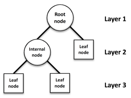
Figure 2. structure of decision tree.

2.4. Support Vector Machine

Support Vector Machine is a two-category classification model that Cortes and Vapnik first proposed in 1995. The learning strategy of SVM is to maximize the interval. Its fundamental model is a linear classifier with the largest interval defined in the feature space[12]. Different from traditional artificial neural networks, SVM not only have simple structure, but also have better technical performance, especially generalization ability. In SVM, hyper planes are selected to best separate dots in the input variable area from their categories. It distinguishes the two tyoes of samples by constructing the classification plane, and then classifies the features extracted from the test samples. The margin is the separation between the hyper planes and the closest data point. The line with the largest margin is the best or ideal hyperplane that can split two categories. Support vectors are the names for these points. Only the support vector plays a role in determining the best hyperplane.

SVM has some advantages. First, when there is a very clear distinction between each class, the classification effect of SVM is relatively good. Second, SVM is more advantageous when the dimensionality of the space is high. Third, SVM is also effective when the dimension is larger than the number of samples[13]. SVM also has some disadvantages. First, a long time is taken by SVMs to train on larger datasets. Second, traditional SVMs are only capable of binary classification, so there are a lot of restrictions on their use. Finally, it is not as easy to learn and understand as decision trees[14].

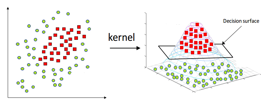
Figure 3. Support Vector Machine.

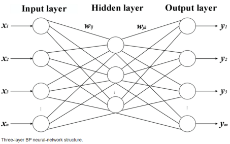
Figure 4. Structure of BP neural network.

2.5. Classical BP neural network

BP neural network is a concept that is proposed by scientists that are led by McClelland and Rumelhart in 1996. It is one of the most uses neural network models widely. Its learning rule is to use the most exorbitant descent method, by using back propagation to adjust the country value and weight of the network constantly, so as to minimize the sum of the network's squared errors. The signal propagates through the forward direction and the error propagates through the back propagation, which is the main characteristic of the bp neural network.

There are several activation functions commonly used in BP neural network, including Sigmoid, Tanh function and Relu function. The sigmoid function is generally used in the hidden layer, which is divided into log-sigmoid function and tan-sigmoid function. These two functions have different output ranges, and the selection of practical applications depends on the requirements. The log-sigmoid function can be obtained by formula.

\( f(x)=\frac{1}{(1+{e^{-x}})} \)

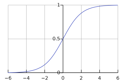
Figure 5. Sigmoid Function.

Tanh function solves the disadvantage that the center of sigmoid is not 0, but it still has the disadvantage that the gradient is easy to disappear. Tanh function can be calculated by this formula.

\( f(x)=\frac{{e^{x}}-{e^{-x}}}{{e^{x}}+{e^{-x}}} \)

Figure 6. Tanh Function.

The relu function is a general activation function, which is improved for the shortcomings of the sigmoid function and tanh.

\( f(x)=max⁡(0,x) \)

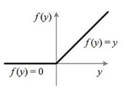
Figure 7. Relu Function.

There are some advantage of BP neural network. First, it is very fast, simple, and easy to analyze and program. Second, this method is flexible and there is no need to acquire more knowledge about the network. Third, this is a standardized method and works very efficiently[15]. There are some drawback of BP neural network. First, the choice of the number of hidden layers and units can only be explored by experience. Second, it can be sensitive for noisy data[16]. Third, the function or performance of the back propagation network on a certain issue depends on the data input.

The feature extraction in the above traditional algorithms relies on the manually designed extractor, which requires professional knowledge and parameter adjustment process. Deep learning is mainly data-driven feature representations of data sets can be obtained, and the expression of data sets is more efficient and accurate.

Conventional Neural Network (CNN) is a kind of feedforward neural network, which is specially designed for image recognition problems. The most different from the general neural network is the addition of convolution layers and pooling layers. The advantages of image classification through the use of conventional neural network are high detection accuracy, fast operation speed and stable detection results. Automatic feature extraction is achieved by simulating the processing mechanism of the brain, making it intelligent.

3. Deep learning based image classification algorithm

3.1. LeNet-5

Professor Yann LeCun proposed the LeNet-5 model in 1998. It was the first convolutional neural network to successfully address a problem of number recognition. Seven layers make up this model, including one fully linked layer, two pooling layers, and three convolution layers.

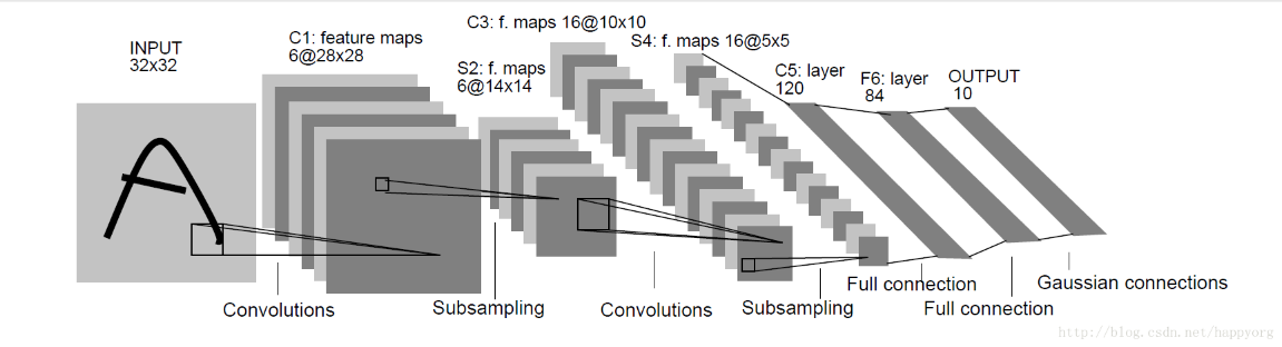
Figure 8. Structure of LeNet-5.

The LeNet-5 model will receive input spreads up to 32*32[17]. With 6 5*5 convolution cores and a 28*28 feature mapping, the C1 convolution layer can prevent information from the input image from escaping the convolution kernel's border. The subsampling layer (S2) is followed by a filter size of 2*2 and length and width steps of 2, resulting in the production of six feature graphs with a size of 14*14. 16 5*5 convolution kernels make up the convolutional layer C3. This layer's input matrix measures 14*14*6. S4 and S2 are similar, 15 feature maps, each measuring 2 by 2, will be produced. 120 convolution kernels of size 5*5 make up the convolutional layer C5. F6 is a completely linked layer that is entirely connected to C5 and produces 84 feature maps in the end. At present,LeNet-5 has been studied in various application tasks such as handwritten character recognition, flow recognition and so on. This network structure can make the input image fit well with the topology of the network and for feature extraction and pattern classification, they will be generated in training at the same time, and the network’s training parameters can be reduced by weight that shares, making the neural network formation more simple-minded and more adaptable. But LeNet-5 is not ideal for dealing with complex problems.

3.2. AlexNet

AlexNet is designed by Hinton and his student Alex Krizhevsky. This network was invented to achieve better ImageNet Challenge results. Eight layers were contained by AlexNet; the first five layers were convolutional, some of them were then followed by layers that used maximum pooling, and the final three layers were fully connected. When compared to tanh and sigmoid, it utilised the non-saturating ReLU activation function, which demonstrated improved training performance[18].

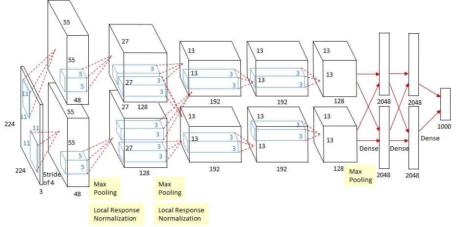
Figure 9. Structure of AlexNet.

The input of AlexNet is a 227*227*3 image, and its production is a 1000-dimensional vector, corresponding with each classification’s probability. To reduce the problem of overfitting, it implements data augmentation, including cropping and flipping images to increase the richness of the training set. In the first layer of AlexNet, the convolution window’s shape is 11*11.The reason for using such a large convolutional window to capture images is because the images in ImageNet are more than 10 times larger than the images in MNIST. Then, after the convolution of the first, wecond and fifth layers, a pooling layer is added, whose Kernel is 3*3 and step size is 2. Such a pooling layer increases the accuracy by about 0.3%. In the second layer, the convolution window's shape is diminished to 5 by 5 and subsequently 3 by 3. There are two fully linked layers following the final convolutional layer, each with 4096 outputs. In AlexNet, changing the activation functions Sigmoid and Tanh to ReLU can greatly solve the problem of vanishing gradient, and the calculation speed is also faster[19]. AlexNet uses RELU as the activation function, which speeds up the convergence. Use dropout to avoid overfitting, but there are 60 million parameters, and the amount of calculation is relatively large.

3.3. VGG

VGG is a standard deep Convolutional Neural Network architecture with multiple layers. Developed as a deep neural network, baselines are also surpassed by the VGG Net on alot of datasets and tasks beyond ImageNet. Furthermore, it still is one of the most popular image recognition architectures now[20]. Compared with the previous AlexNet, VGG has a deeper depth, more parameters (138 million), and better effect and portability.

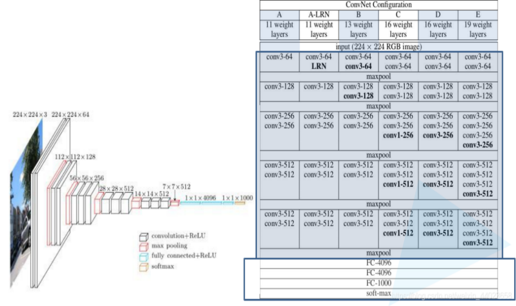
Figure 10. Structure of VGG.

VGG is divided into VGG-16 and VGG-19. VGG-16’s structure is shown in column D of the figure and VGG-19’s structure is shown in column E of the figure. There is no essential difference between the two, only the depth of the network is different. The design of various VGG networks is very unified, with the same 224*224*3 input + 5 maxpool layers + 3 FC fully connected layers. The VGG network's topology is also quite consistent, as it uses 3*3 convolution and 2*2 maxpooling throughout. The main difference is the middle VGG Block are designed differently. In VGG, in order to keep the image size consistent, the size of all image inputs is 224x224. In convolution layers then use a minimal receptive field, the smallest possible size stilling left/right and captures up/down. Furthermore, there are also 1*1 convolution filters performing the role of a linear transformation of the input. The hidden layers in VGG Network are all use ReLU. Local Response Normalization is not usually leveraged (LRN) by VGG as it increases training time and memory consumption. Last, there are three fully connected layers in VGG Network. VGG can be used in face recognition, image classification, etc. Although the structure of VGG Net is very compact and Several tiny (3x3) convolutional layer combinations perform better than a single large (5x5 or 7x7) convolutional layer because VGG requires more processing power and uses more parameters, which increases memory usage[21].

4. Experiment and performance analysis

4.1. Common image classification datasets

The following are several commonly used classification data sets based on conventional neural networks, mainly including the MNIST, CIFAR-10 and ImageNet.MNIST[22] data set is one of the most studied data sets in computer vision and machine learning literature. The foal of this data set is to correctly classify the handwritten numbers 0-9. It contains 60,000 training pictures and 10,000 test pictures. CIFAR-10 is another standard reference data set in the computer vision and machine learning literature. It contains 60,000 colour images, of which 50,000 are for training and 10,000 for testing. These photos are divided into 10 categories, 6,000 in each category. ImageNet a large visual database with more than 14 million colour images. It contains more than 20,000 categories. This data set is still one of the most commonly used data sets for image classification, detection and positioning in the field of deep learning.

4.2. Evaluating indicators

Generally, confused matrices can be used to predict results. Confusing matrix is standard format for representing accuracy evaluation, which is represented in the matrix form of n rows and n columns. Among them, rows represent real values and columns represent predicted values. By using the single results predicted by the confusion matrix, we can calculated the four evaluation indicators of accuracy, recall rate, accuracy rate and F1 score from the data in the chart.

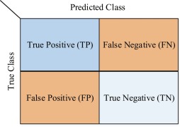
Figure 11. Confusing Matrix.

(1) Accuracy is defined as the proportion of samlpes properly identified by the classifier to all sample books for a particular test data set, which can be obtained by the following calculation formula:

\( accuracy=\frac{TP+TN}{TP+TN+FP+FN} \)

(2) Precision is the ratio of all correctly classified positive examples to all positive examples correctly categorized as positive examples, which expresses the proportion of all correctly predicted results to all observations and gauges the retrieval system's precision rate. It can be calculated by the following formula:

\( precision=\frac{TP}{TP+FP} \)

(3) Recall, which measures the retrieval system's recall rate, is the proportion of correctly identified positive examples to the actual number of positive examples. It can be obtained by the following formula:

\( recall=\frac{TP}{TP+FN} \)

(4) The F1 score is an indicator of balanced performance. Because of the advantage, we not only pay attention to the accuracy of positive samples, but also care about the recall rate, but do not want to measure it with the accuracy rate, so we can use the F1 score. F1 score can be obtained by the following formula: \( F1-score=\frac{2×precision×recall}{precision+recall} \)

4.3. Performance comparison

Table 1. Compare each methods’ accuracy.

According to the table, compared to KNN and SVM, the accuracy of decision tree and naive Bayes in the MNIST dataset is not as good as that of KNN and SVM. The accuracy rates of KNN and SVM both exceed 95%. So it will be better to use KNN or SVM when it is used to distinguish yes or no.

5. Discussion

At present, there are still many shortcomings in the field of image recognition. In order for the model to still have a decent generalization ability for scenes that have never appeared before, it is first important to improve its generalization ability. Because the test image can originate from a different data distribution in practice than it did during training. There may be several ways in which the training data and this previously unseen data diverge. Deep network models' accuracy will decline as a result of this disparity in data distribution[23]. Second, in the field of artificial intelligence, although image recognition has the ability of high definition and information processing, there are still large errors in data processing. Because image recognition technology has a variety of advantages such as information acquisition and information utilization, its effective application in image processing can ensure the accuracy of information processing while improving the processing scheme. Image processing technology has become the direction of future artificial intelligence. Technicians should improve software technology and hardware technology according to different application scenarios.

6. Conclusion

Image recognition has always been a research hotspot in the field of computer vision. It has been applied in many fields such as face recognition, traffic scene recognition and aerial remote sensing. Based on the traditional image recognition framework based on manual features and the depth image recognition framework based on convolutional neural network, this paper introduces and analyzes the representative algorithms in the field of image recognition. In addition, common image recognition data sets and evaluation indexes are introduced, and the results of representative methods are compared quantitatively. Finally, we summarize the existing research problems in the field of image recognition and discuss the possible future development of this field.

References

[1]. Fix, Evelyn, and J. L. Hodges. “Discriminatory Analysis. Nonparametric Discrimination: Consistency Properties.” International Statistical Review / Revue Internationale de Statistique, vol. 57, no. 3, 1989, pp. 238–47. JSTOR, https://doi.org/10.2307/1403797. Accessed 29 Aug. 2022.
[2]. N. S. Altman (1992) An Introduction to Kernel and Nearest-Neighbor Nonparametric Regression,The American Statistician, 46:3, 175-185, DOI: 10.1080/00031305.1992.10475879
[3]. Bandan, Sheikh. (2022). Re: What are some advantages of kNN algerthim? Retrieved from: https://www.researchgate.net/post/What_are_some_advantages_of_kNN_algerthim/6256904b4004ac3a617fe44b/citation/download.
[4]. http://theprofessionalspoint.blogspot.com/2019/02/advantages-and-disadvantages-of-knn.html
[5]. Naive Bayes in Machine Learning | How Naive Bayes works? (educba.com)
[6]. https://www.quora.com/What-are-the-disadvantages-of-using-a-naive-bayes-for-classification
[7]. https://www.jianshu.com/p/b64b7373e3fd
[8]. https://scikit-learn.org/stable/modules/tree.html#:~:text=Decision%20Trees%20(DTs)%20are%20a,as%20a%20piecewise%20constant%20approximation
[9]. https://dhirajkumarblog.medium.com/top-5-advantages-and-disadvantages-of-decision-tree-algorithm-428ebd199d9a
[10]. Cortes, C., Vapnik, V. Support-vector networks. Mach Learn 20, 273–297 (1995). https://doi.org/10.1007/BF00994018
[11]. https://dhirajkumarblog.medium.com/top-4-advantages-and-disadvantages-of-support-vector-machine-or-svm-a3c06a2b107
[12]. https://statinfer.com/204-6-8-svm-advantages-disadvantages-applications/
[13]. http://theprofessionalspoint.blogspot.com/2019/03/advantages-and-disadvantages-of-svm.html
[14]. https://www.watelectronics.com/back-propagation-neural-network/#:~:text=Advantages%2FDisadvantages,more%20knowledge%20about%20the%20network.
[15]. https://mulloverthing.com/what-are-the-advantages-and-disadvantages-of-backpropagation/#What_are_the_advantages_and_disadvantages_of_backpropagation
[16]. https://en.wikipedia.org/wiki/LeNet
[17]. Alex Krizhevsky, Ilya Sutskever, and Geoffrey E. Hinton. 2017. ImageNet classification with deep convolutional neural networks. Commun. ACM 60, 6 (June 2017), 84–90. https://doi.org/10.1145/3065386
[18]. https://www.bilibili.com/read/cv7905812/
[19]. Read more at: https://viso.ai/deep-learning/vgg-very-deep-convolutional-networks/
[20]. https://blog.csdn.net/weixin_44957722/article/details/119089221
[21]. G. Cohen, S. Afshar, J. Tapson and A. van Schaik, "EMNIST: Extending MNIST to handwritten letters," 2017 International Joint Conference on Neural Networks (IJCNN), 2017, pp. 2921-2926, doi: 10.1109/IJCNN.2017.7966217.
[22]. https://zhuanlan.zhihu.com/p/470662008
Cite this article
Zhuang,Y. (2023). Researches advanced in image recognition. Applied and Computational Engineering,4,205-214.
Data availability
The datasets used and/or analyzed during the current study will be available from the authors upon reasonable request.
Disclaimer/Publisher's Note
The statements, opinions and data contained in all publications are solely those of the individual author(s) and contributor(s) and not of EWA Publishing and/or the editor(s). EWA Publishing and/or the editor(s) disclaim responsibility for any injury to people or property resulting from any ideas, methods, instructions or products referred to in the content.
About volume
Volume title: Proceedings of the 3rd International Conference on Signal Processing and Machine Learning
© 2024 by the author(s). Licensee EWA Publishing, Oxford, UK. This article is an open access article distributed under the terms and
conditions of the Creative Commons Attribution (CC BY) license. Authors who
publish this series agree to the following terms:
1. Authors retain copyright and grant the series right of first publication with the work simultaneously licensed under a Creative Commons
Attribution License that allows others to share the work with an acknowledgment of the work's authorship and initial publication in this
series.
2. Authors are able to enter into separate, additional contractual arrangements for the non-exclusive distribution of the series's published
version of the work (e.g., post it to an institutional repository or publish it in a book), with an acknowledgment of its initial
publication in this series.
3. Authors are permitted and encouraged to post their work online (e.g., in institutional repositories or on their website) prior to and
during the submission process, as it can lead to productive exchanges, as well as earlier and greater citation of published work (See
Open access policy for details).