1. Introduction

The improvement of the quality of life marks the progress of civilization. As the garbage segregation movement rolls out everywhere as an ordinance that advocates everyone to implement it, many people desire something like a smart app to help them identify and categorise garbage as it is easily misidentified and misclassified. Commuters or workers whose lives are squeezed by the pressures of work urgently need to reduce the amount of time they spend in this, and others are tired of having to constantly check the standard of garbage classification since they may be fined for mistakes. Some pieces of Chinese news have reported on the lack of knowledge about waste separation among the general public and the penalties it brings. For example, in a municipal survey report in June 2015, 2,370 garbage sorting problems were found in 165 living communities in Hangzhou, among which 1,631 problems such as wrong garbage throwing and wrong sorting accounted for 68.82% of the total number of problems, topping the list [1]. Even in 2022, three-fifths of the people interviewed at random on the street cannot answer the question about waste separation.

In summary, it would be useful to design a program that intelligently identifies images to select their attribution. The step of identifying the type of garbage in the process of classification is the most important. A machine learning-based approach would be the most appropriate choice, due to its accuracy and stability that would be trustworthy when trained correctly. For the image recognition task, the best performing deep learning algorithm is the Convolutional Neural Network (CNN). On the one hand, it reduces the number of weights making the network easy to optimize. On the other hand, it reduces the complexity of the model and reduces the risk of overfitting. In image processing tasks, CNN avoids the complex process of feature extraction and data reconstruction in traditional recognition algorithms and is able to compress a huge amount of pixel information without losing its features, making it suitable for high-resolution garbage photo processing work [2]. This also significantly reduces the computational pressure on program operation.

In this study, the dataset obtained from the website Kaggle was used as training [3]. The experimental results are positive, the accuracy of recognition is high and the task of classification is excellently performed. In addition, several methods have been proposed to improve some detailed flaws of the training process. A cost function is used to measure the deviation of the model prediction and the weight settings are updated using gradient descent and back propagation. The resulting value of cost was able to converge to a minimum overall, but had the problem of continuous floating during the descent. It is expected that the model can perform better with a suitable learning rate descent adjustment.

2. Method

2.1. Data Preparation

Table 1. Number of Images for each class.

The data are found on Kaggle Garbage Classification Dataset [3]. The datasets are made up by 2, 467 images as a total and divided into 6 classes, which are cardboard, glass, metal, paper, plastic and other trash. We used 2019 images for training the model, 252 images for validating and 256 images for testing. The number of images is covered in Table 1 Moreover, augmentation operations are done, such flipping to the right and left, in order to make the effects of some factors unrelated to image recognition as little as possible, thereby making the model more stable and run well.

2.2. CNN model

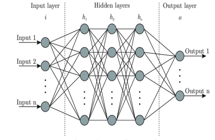
Since the project is based on the recognition of images of trash, it is determined to use CNN, one kind of artificial deep learning neural network shown in Figure 2 which consists of some layers such as nonlinear, pooling, and fully connected layers shown in Figure 1 [4]. The efficiency of CNN in image classification is remarkably high. We build our program on Jupyter Notebook, with the framework TensorFlow, and our optimizer is ADAM. The default learning rate of TensorFlow is 0.001. The ADAM function ensures the adaptive learning rate, so the learning rate will not keep constant [5]. The varying learning rate ensures the efficiency of finding gradients using gradient descent technique, thus we averagely use 140 seconds for training each epoch and the total time used for finishing 64 epochs is about 2.5 hours. However, if the SVG optimizer is applied, the running time maybe twice longer. After training the model, accuracy was noted. In addition to models’ accuracy, the training loss and validation loss were also noted.

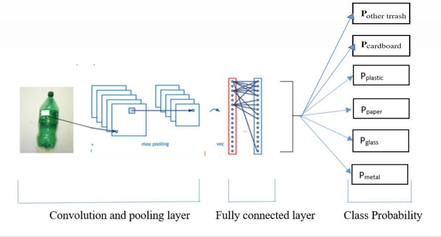
The process of convolution is using a trainable filter for convoluting an input image. At the first layer, images are input. Next, after the convolution with kernel size 3×3, features of the images are extracted to form a feature map with the size 3×3. Due to the shrinkage of pictures, it can be regarded as the loss of data. Therefore, we apply a padding layer, filling the feature map to make the output size consistent with the size of the input images [7]. Then then data will pass through the max pooling layer, with size 2×2. It would reduce the dimensionality of the feature maps by extracting the useful details and discarding unrelated images. More concretely, it slides through the feature map and divides it into 2×2 matrices repeatedly. Later the maximum number in each matrix is chosen, which would decrease 75% amount of data. In simple terms, pictures are compressed, and main parameters are get, thus improving the efficiency of the model [8]. The subsequent padding layer does the same role as it did in the former layer. The later layer is the flatten layer. It is a concrete operation to enter fully connected neural network in Keras framework. In simple words, the concept of flattening is straightening and pressing. The high-level image abstractions obtained by convolution and pooling are flattened into one-dimensional vectors. After continuous abstraction of image data, network parameters are greatly reduced. However, the one-dimensional vectors retain the essential key information [9]. Finally, it comes in to two dense layers. Due to the truth that most data in real world are nonlinear, dense layers with activation functions can extract the features in front of the dense after nonlinear changes and extract the relationship between these data and finally exhibite the relationship of these processed data [10]. This process is also a convolution operation, and the operation of convolution comes from the principle of vector dot products. At the first dense layer, we use Relu as the activation function. The reason for using Relu is that the gradient would easily disappear when activation function, Sigmoid, is propagating. When the Sigmoid function is approaching the saturation point, the derivative of the function will be zero. This makes the program not works properly. However, Relu function fixes the problem of the disappearance of gradient, and it reduces the dependence among parameters. Therefore, it takes less computation time and faster compared with Sigmoid [10]. The gradient of Relu only takes two values: 0 and 1. If the input number is negative, the output gradient will be zero and when the input is positive, it would take one as the gradient. [10, 11]. The so second dense layer is used with the activation function Softmax. It helps to normalize vector to probability distribution vectors. Moreover, Softmax function is efficient in multi-classes classification [6], which is beneficial in our trash classification that involves 6 classes trash. Table 2 presents the structure of the model used in the study.

Table 2. Parameters at Each Layer.

3. Results and Discussion

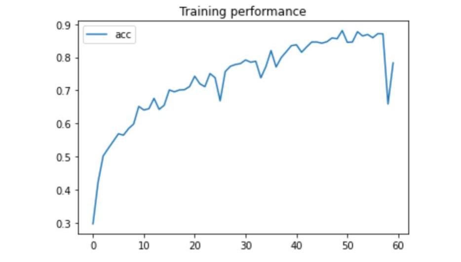
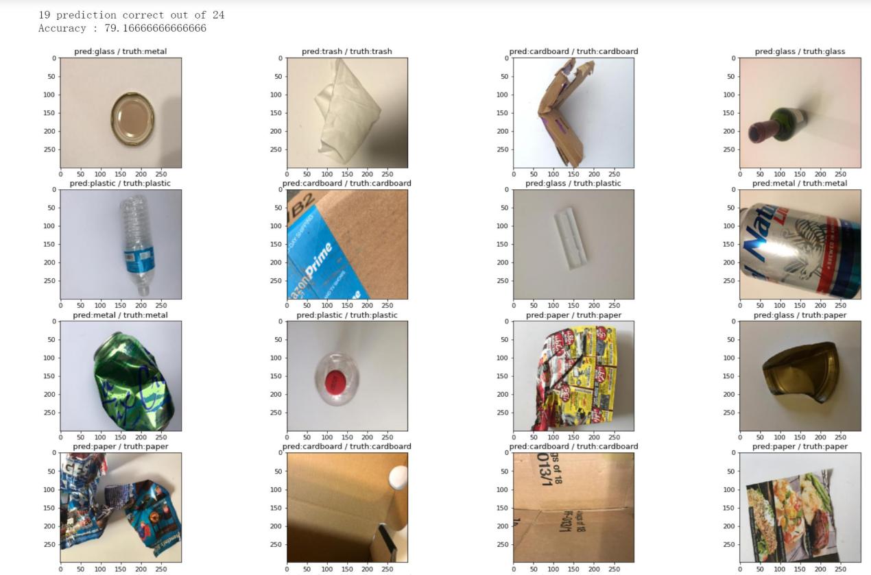
We set 64 epochs of training and validating, and finally we also chose some pictures to do the testing process to check if the program can distinguish the trash in correct labels. After training the model, accuracy is marked in Figure 4. In addition to accuracy of model training, the loss of training and validating are also marked in Figure 3. The testing accuracy is noted in Figure 5, with which the comparation of results of prediction and the truth of the trash can be apparently seen. The figures demonstrate our model is getting better as the loss is declining and the accuracy is increasing progressively. From the previous research, we see Thung and Yang has created a Convolutional Neural Network to sort 6 categories of trash, and our 6 trash classes are the same to theirs [12]. Thung and Yang’s CNN model can achieve 73% accuracy at their sorting process [12]. But as we can see from Figure 3, our accuracy can almost reach more than 85%, and the training loss can be lower than 0.4. Moreover, the lowest loss of validation can be 0.75 and averagely 0.802 after 30 epochs. The accuracy of validation can be up to 0.78. We draw the pictures of prediction of on single batch of testing, which includes 24 images of trash. According to Figure 5, the correct rate can be 19 out of 24, which is an accuracy about 79%.

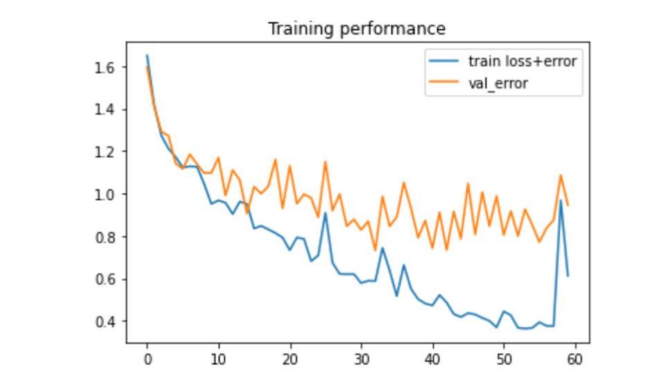
The program is learning linearly, and it has a little bit fluctuation. The reason lies in the fact of ADAM optimizer which takes the adaptive learning rate to finds the local minimum. It is reasonable. If we set the learning rate at the very beginning and only applied the unchangeable learning rate, it would be too aggressive so the CNN may exist erratic behavior or it would be too small making a long time to train the model. Besides, due to our relatively large number of convolution operations, the features of the trash images are extracting well and learn by the model almost accurately. Therefore this paper can obtain such a high accuracy.

At the last epoch, the accuracy suddenly drops down may due to the small number of images that causes over-fitting. Also, it is a reasonable fluctuation which can be solved for more iterations and learning. Besides, the accuracy of testing can be improved for clearer images.

4. Conclusion

An approach based on CNN, the deep learning algorithm has been devised. By compressing the accuracy of the images while preserving the key information, the computational and learning pressure of the model is greatly reduced. After completing the convolution process, the model is trained. The test results show that this model predicts more accurately and has lower loss values than the previous CNN models made by previous researchers that do the same task. The model can be further optimized. Specifically, since an automatically adjusted learning rate has been applied, there are fluctuations in the loss descent process presented by the program. Moreover, the small number of image samples raises the problem of overfitting, making the test accuracy appear significantly lower after the number of training iterations becomes larger. Therefore, it is planned to continue improving the model in the future. More samples will be obtained, the number of iterations will be increased on top of that, and the model will be further extended to make it possible to categorize the waste after identifying the type of it for guidance on drop-off and recycling disposal. Hardware with more computing power will also better support the project. The model will be put into practice to improve the motivation of citizens to separate waste by making the implementation process easier. This will help the community to better sort their waste and improve the quality of life.

References

[1]. Hangzhou Daily, 2015, retrieved from https://huanbao.bjx.com.cn/news/20150716/642650. Shtml.
[2]. Gyawali D et al. 2020. Comparative analysis of multiple deep CNN models for waste classification. arXiv preprint arXiv:2004.02168.
[3]. Kaggle. 2018. Garbage classification. https://www.kaggle.com/datasets/asdasdasasdas/garbage-classification
[4]. Albawi S 2017. Understanding of a convolutional neural network. In 2017 international conference on engineering and technology (ICET) (pp. 1-6). Ieee.
[5]. Kingma D P 2014. Adam: A method for stochastic optimization. arXiv preprint arXiv:1412.6980.
[6]. Sharma S et al. 2017. Activation functions in neural networks. towards data science, 6(12), 310-316.
[7]. Analyticsindiamag 2021. Guide to Different Padding Methods for CNN Models, https://analyticsindiamag.com/guide-to-different-padding-methods-for-cnn-models
[8]. Cnblog. Studying for pooling layer. www.cnblogs.com/MrSaver/p/10356695.html
[9]. Jeczmionek E. 2021. Flattening Layer Pruning in Convolutional Neural Networks. Symmetry, 13(7), 1147.
[10]. Analyticsindiamag 2021. Guide to Different Padding Methods for CNN Models, https://analyticsindiamag.com/guide-to-different-padding-methods-for-cnn-models
[11]. Brosch T 2016 et al. Deep 3-D convolutional encoder networks with shortcuts for multiscale feature integration applied to multiple sclerosis lesion segmentation. IEEE Trans Med Imaging 35(5):1229–1239
[12]. Yang M 2016 Classification of trash for recyclability status. CS229 project report, 2016(1), 3.
Cite this article
Chen,Y.;He,Y.;Lin,J.;Sun,S. (2023). Garbage image recognition and classification based on CNN. Applied and Computational Engineering,4,416-421.
Data availability
The datasets used and/or analyzed during the current study will be available from the authors upon reasonable request.
Disclaimer/Publisher's Note
The statements, opinions and data contained in all publications are solely those of the individual author(s) and contributor(s) and not of EWA Publishing and/or the editor(s). EWA Publishing and/or the editor(s) disclaim responsibility for any injury to people or property resulting from any ideas, methods, instructions or products referred to in the content.
About volume
Volume title: Proceedings of the 3rd International Conference on Signal Processing and Machine Learning
© 2024 by the author(s). Licensee EWA Publishing, Oxford, UK. This article is an open access article distributed under the terms and
conditions of the Creative Commons Attribution (CC BY) license. Authors who
publish this series agree to the following terms:
1. Authors retain copyright and grant the series right of first publication with the work simultaneously licensed under a Creative Commons
Attribution License that allows others to share the work with an acknowledgment of the work's authorship and initial publication in this
series.
2. Authors are able to enter into separate, additional contractual arrangements for the non-exclusive distribution of the series's published
version of the work (e.g., post it to an institutional repository or publish it in a book), with an acknowledgment of its initial
publication in this series.
3. Authors are permitted and encouraged to post their work online (e.g., in institutional repositories or on their website) prior to and
during the submission process, as it can lead to productive exchanges, as well as earlier and greater citation of published work (See
Open access policy for details).