1. Introduction

Emotion is a unique attribute of human beings. It is an important driving force for us to recognize the world and act. It plays a key role in interpersonal communication and social interaction. In recent years, with the rapid development of artificial intelligence technology, emotion recognition has become one of the core technologies to promote artificial intelligence to human-computer interaction naturalness and strong artificial intelligence. Although the traditional AI system performs excellently in logical reasoning and data processing, it is difficult to perceive and understand the human emotional state, which seriously restricts the deep investment and application of AI in the fields of education and medical treatment. In this context, exploring efficient and accurate emotion recognition methods will become a research focus in the future.

Nowadays, the mainstream method of emotion recognition is to analyze the directly collected human physiological signals to ensure the objectivity of emotional information. These signals include EEG, EOG, ECG, etc. In recent years, most researchers have used traditional machine learning and deep learning for emotion recognition based on EEG. In traditional machine learning, some research based on frequency domain feature extraction and SVM model can achieve an accuracy of about 91.7% [1]. In terms of deep learning, CNN and LSTM models and their variants are the most mainstream in the field of EEG emotion classification [2, 3, 4]. Among them, the research based on GCN model and its optimization model has achieved an accuracy rate of more than 90% [5, 6, 7]; The research based on LSTM model and its variants has also made considerable achievements [8, 9]; Based on the experiments of CNN and LSTM models [10, 11, 12], they achieved 80%-98% accuracy in DEAP [13], SEED, SEEDV and other data sets. However, the process of continuous optimization of the model, often means more complex model architecture and parameters that need to be constantly debugged. Researchers will spend a lot of time to find the optimal parameters. At present, the main methods to find parameters are grid search [14, 15], random search, etc. These algorithms will consume a lot of resources, so this paper proposes a method to find the optimal combination of super parameters based on reinforcement learning, and verifies the effect of this method through emotion recognition based on EEG.

2. Dataset and preprocess

2.1. DEAP dataset

DEAP is a public multimodal emotion recognition data set built by Koelstra et al. In 2012 [15]. It synchronously collected EEG signals and peripheral physiological signals of 32 subjects while watching 40 music videos, and combined with subjective emotion score, established a complete mapping relationship between emotion induction, physiological response and subjective feedback. The DEAP dataset consists of two parts. One is a database of 120 one-minute music videos. Each video is scored by 14-16 volunteers according to potency, arousal and dominance. The other is a subset of the former, which is composed of 40 Music Videos. Each video has the corresponding EEG and physiological signals of each participant in the 32 participants. Each video is scored according to potency, arousal and dominance dimensions. The second part of the DEAP data set is used in this paper. Figure 1 shows the distribution of electrode plates and Arousal-Valence model of emotions.

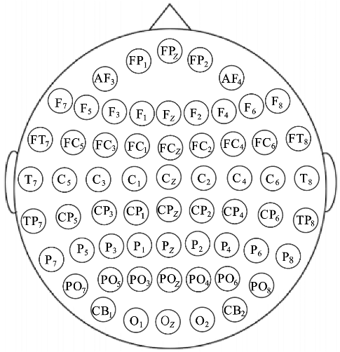
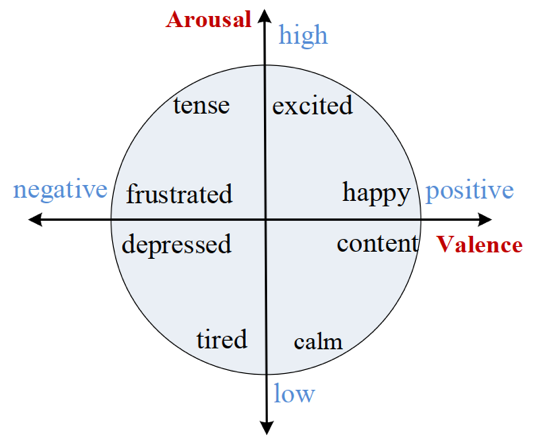
Figure 1: Arousal-valence model of emotions and electrode distribution for EEG signal acquisition [15]

The original data in the DEAP dataset contains preprocessing information for each of the 32 participants, including data and labels. The data is a 40 x 40 x 8064 array, including 8064 time points of each channel in 40 channels and each channel in 40 Music Videos (experimental time 63s × sampling frequency 128Hz). The tag is a 40 x 4 array, containing the potency, wake-up, domination and link notes of each of the 40 Music Videos.

2.2. Dataset preprocessing

In this paper, eight non-EEG signals such as EMG and ECG are eliminated to prevent the influence of irrelevant signals on the experimental results. The processed data shape is (328064). Then, this paper reduces the dimension of the relevant data from 8064 time points to 99 statistical features, and changes its shape to (32, 99). Specifically, the 8064 time points of each EEG channel are first divided into 10 batches, including 9 batches containing 807 time points and one batch containing 801 time points. Then, calculate 9 Statistics (mean, median, maximum, minimum, standard deviation, variance, range, skewness, kurtosis) for each batch, and make the first 90 characteristics of each channel come from 10 batches × 9 statistics. Finally, calculate the same 9 statistics for all 8064 time points of each channel, so that each channel gets 90 (batch characteristics) + 9 (global characteristics) = 99 characteristics. Then, each sample feature should be standardized one by one, specifically through the following formula (1).

\( {x_{i}}=\frac{{x_{i}}-mean({x_{i}})}{std({x_{i}})}\ \ \ (1) \)

Where \( {x_{i}} \) is a statistic, and the value range of I is [1,9]. Finally, this paper extracts the first two tags of each experiment, packs them and the processed data into a dictionary, serializes them into .dat files through pickle, and stores them in the target directory.

3. Methods

3.1. Deep learning

In this experiment, the CNN model uses a three-layer convolution structure for feature extraction and classification of EEG signals, and its specific structure is shown in Figure 2.

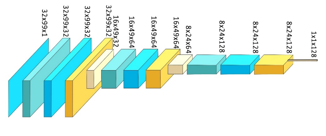
Figure 2: CNN model structure (picture credit: original)

The input layer of the model is EEG data of (batch, 1, 32, 99), which corresponds to 32 electrode channels and 99 time points. The first convolution layer uses 32 (3 × 5) cores, maintains the size of the feature map through (1,2) symmetrical filling, and cooperates with the LeakyReL activation function and (2 × 2) maximum pooling. The main function of this layer is to capture the local temporal and spatial characteristics of the original EEG signal; In the second layer, 64 (3 × 3) convolution cores are used to reduce the pooled feature map to 8 × 24, retain the key time dynamic information and suppress noise interference; The third layer is extended to 128 channels to maintain the resolution of the feature map. Then, the spatial dimension is compressed to (1 × 1) by global average pooling. Then, the dropout layer is added in front of the full connection layer. This layer randomly closes some neurons depending on the dropout probability input, so that the network can avoid excessive dependence on specific local features, inhibit the over fitting of the model and enhance the generalization ability. Finally, after a full connection layer outputs the predicted value, the weighted moments of the full connection layer combine the 128 dimensional features to generate the non-normalized classification scores (Logits). Combined with the loss function (BCEWithLogitsLoss), this layer directly outputs the discrimination value of binary classification task, and converts it into probability through sigmoid function.

3.2. Reinforcement learning

3.2.1. Complete process

This experiment realized automatic parameter adjustment mainly through reinforcement learning environment module, agent module, and model training module. The specific process is shown in Figure 3.

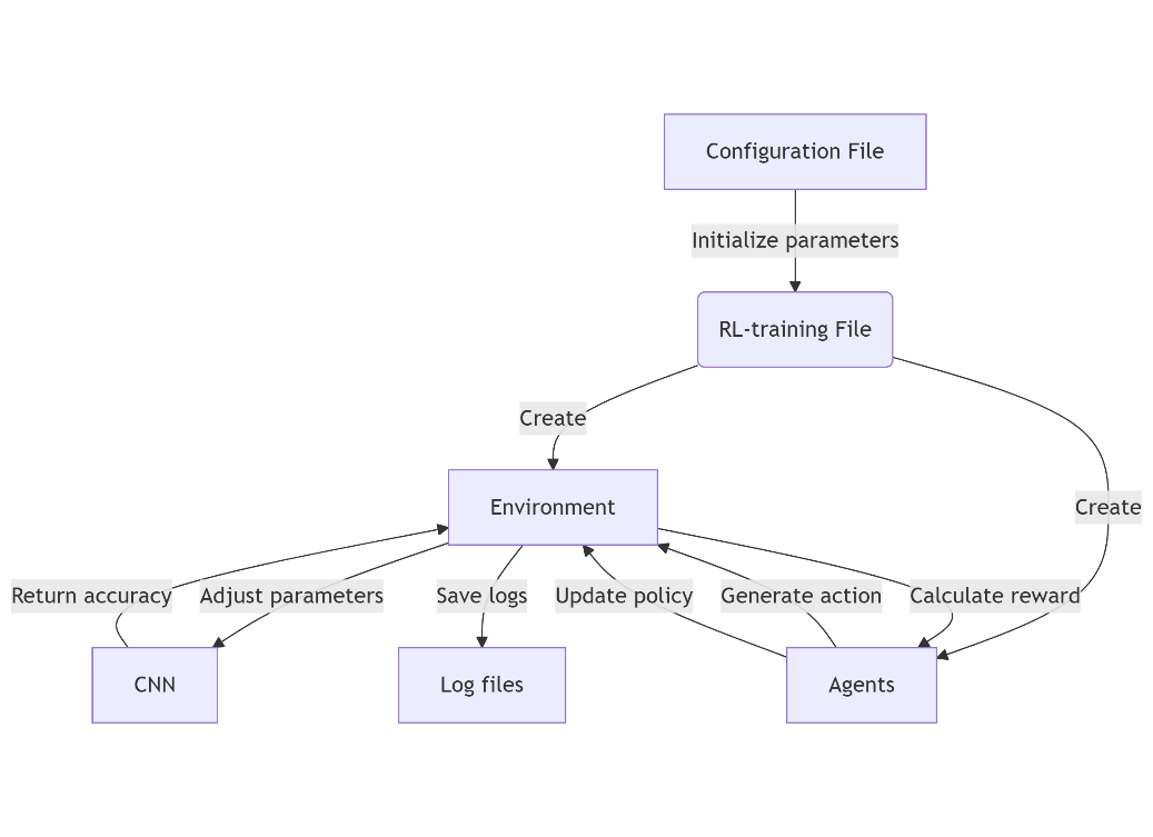
Figure 3: Reinforcement training process (picture credit: original)

3.2.2. Environment construction

In the construction of reinforcement learning environment, the core goal is to optimize the accuracy of the model in emotion recognition tasks by dynamically adjusting the hyper parameters of the deep learning model. The environment defines the state space, action space, and reward mechanism, and works with PPO algorithm or DDPG algorithm.

The state space is composed of hyperparameters, specifically including learning rate (LR), dropout probability (dropout_prob) and batch_size, which are encoded into three-dimensional vectors by normalization. This design enables the agent to perceive the characteristics of the current parameter combination and provide the basis for its decision. The mathematical expression of the state vector is shown in formula (2).

\( v=[lr , dropout\_prob , batch\_size]\ \ \ (2) \)

Among them, the value range of dropout probability and batch size is dynamically mapped to the preset interval through sigmoid function. (in this experiment, the dropout probability is 0.2 – 0.5, and the batch size is 64 – 128)

In the action space, because this experiment only optimizes the dropout probability and batch size, the PPO environment will generate two-dimensional continuous action vectors through the agent, adjust the dropout probability in the first dimension, and adjust the batch size in the second dimension. Through nonlinear mapping, the action value is converted into actual parameters. The batch size adjustment formula (3) is as follows.

\( batch\_size=batch\_min×{(\frac{batch\_max}{batch\_min})^{σ(x)}}\ \ \ (3) \)

In the formula, σ(x) is a Sigmoid function, batch_max and batch_min are the upper and lower limits of the batch size range set in advance. This mechanism ensures the smooth adjustment of movement and avoids the instability of training caused by parameter mutation.

Unlike PPO, the DDPG environment maps the continuous action values (range [-1,1]) output by the agent directly to the preset hyperparameter range (Dropout probability 0.2-0.5, batch size 64-128) through a linear scaling function. The specific formula (4) is as follows.

\( param=min\_val+\frac{action+1}{2}×(max\_val-min\_val)\ \ \ (4) \)

Where param is the final calculated parameter value, max_val and min_val are the upper and lower limits of the parameter value range respectively, and action refers to the action value output by the reinforcement learning agent, usually standardized to the range of [-1,1].

Next, the construction process of the reward mechanism will be explained. The reward section consists of three parts, with the most important being the accuracy improvement reward ( \( {r_{acc}} \) ). If the accuracy of the current training cycle model exceeds the historical best value, a positive reward will be given and multiplied by a coefficient of 20 to amplify the incentive signal of the accuracy change and accelerate the convergence of the strategy. The specific reward formula (5) is as follows.

\( {r_{acc}}=20×({acc_{t}}-{acc_{best}})\ \ \ (5) \)

Where \( {acc_{t}} \) is the accuracy obtained in the current round, \( {acc_{best}} \) is the best accuracy in historical rounds.

Then is the exploration reward ( \( {r_{diversity}} \) ). In order to avoid the agent falling into local optimum, the standard deviation of dropout probability ( \( {σ_{dropout}} \) ) is introduced into the reward function to test the diversity of parameters, see formula (6) for details.

\( {r_{diversity}}=0.1×{σ_{dropout}}\ \ \ (6) \)

This reward encourages agents to explore different parameter combinations to enhance the robustness of the strategy.

Then there is breakthrough reward ( \( {r_{breakthrough}} \) ). Because the accuracy rate will rise and stagnate in the experiment, that is, causing a periodic threshold. Therefore, this incentive is designed to encourage agents to break the threshold, as shown in formula (7).

\( {r_{breakthrough}}=0.5×({acc_{t}}-{acc_{stasis}})\ \ \ (7) \)

Where \( {acc_{t}} \) refers to the accuracy of the current episode, \( {acc_{stasis}} \) refers to the periodic threshold.

Finally, the total reward is the weighted sum of the above components, and the calculation method is shown in formula (8).

\( {r_{total}}={r_{acc}}+{r_{diversity}}+{r_{breakthrough}}\ \ \ (8) \)

3.2.3. PPO agent

PPO agent realizes strategy optimization through actor critical framework, which is mainly composed of an actor network, critical network and experience playback buffer.

In the actor network, the environmental parameters of the current state will be input. Then, the network generates a mean and standard deviation, and then samples from the Gaussian distribution as shown in formula (9).

\( a~N(μ, {σ^{2}})\ \ \ (9) \)

If the current state ( \( {s_{t}} \) ) is given, \( μ \) and \( σ \) will be output by the Actor network, where \( μ({s_{t}}) \) refers to the mean value of the output and \( σ({s_{t}}) \) refers to the standard deviation of the output. Finally, a continuous action ( \( a \) ) will be generated.

The input information accepted in the critical network is the same as that of the actor network. At the output layer, the network will first predict the possible rewards of the current state (hyperparameter combination) and output the corresponding state value.

The output results of the actor critical framework will be stored in the experience buffer for subsequent policy updates. The track data stored includes status, action, reward, logarithmic probability, status value, and termination flag.

Finally, the framework uses Adam optimizer to balance the stability and exploratory of the strategy update by combining the learning rate (0.0005), shear ratio (0.2), entropy regularization coefficient (0.2) and other parameters.

3.2.4. DDPG agent

The main differences between DDPG agent and PPO agent lie in the action generation mechanism, network architecture and update strategy. However, there are still many similarities between them. The implementation method of DDPG agent will be briefly introduced in the following.

The action generation mechanism of DDPG agent adopts deterministic strategy. The actor network directly outputs the continuous action value, and then explores by adding Gaussian noise. The noise decays with training, and gradually reduces the randomness to balance exploration and utilization.

In terms of network architecture, DDPG uses dual target networks, one is actor critical online networks, and the other is a target networks. Through soft update, the two networks gradually synchronize parameters, as shown in formula (10).

\( {θ_{target}}=τ{θ_{online}}+(1-τ){θ_{target}}\ \ \ (10) \)

Where \( {θ_{target}} \) and \( {θ_{online}} \) are the parameter values of target network and online network respectively, \( τ \) is the soft update factor, which is set to 0.005 in the experiment.

Finally, the critical network part obtains the target Q value calculated by the target network by minimizing the timing difference error update strategy, and the actor network part performs the action of maximizing the target Q value predicted by the critical.

3.2.5. RL training

The training process of reinforcement learning is mainly divided into initialization and training models with dynamic parameters. Next, take the training process of PPO as an example.

First import the created reinforcement learning environment (3.2.2) and PPO agent (3.2.3) for initialization, then import the YAML configuration file (4.1) for initialization of hyperparameters. Then, in each episode, the agent generates action vectors according to the current state (hyperparameter configuration) and maps the actions to specific parameter values. Then, the dynamic parameters are imported into the CNN training function to perform 180 rounds of supervised learning. Finally, the accuracy of the validation set is returned as environmental feedback. Among them, the training episodes of reinforcement learning are set to 15 times, which can ensure that the parameter combination can be adjusted to the optimal to a certain extent.

4. Result analysis

4.1. Initial parameter configuration

In the basic CNN experiment, the hyperparameters and training settings required for deep learning are uniformly managed through YAML configuration files. After the configuration file is parsed by the YAML module, the parameters are dynamically injected into the data loading, model construction and optimizer initialization process to ensure the repeatability of the experiment and the traceability of the parameters.

In the automatic parameter adjustment method of reinforcement learning, in order to make the basic deep learning form a control experiment, the initialization parameters of the first episode are the same as those of the basic CNN experiment. The agent added will automatically adjust the two important parameters of dropout probability and batch size in the configuration file in the subsequent episodes, and the other hyperparameters will remain unchanged in each experiment. The initial configuration information is shown in Table 1.

Table 1: Initial configuration

4.2. Result

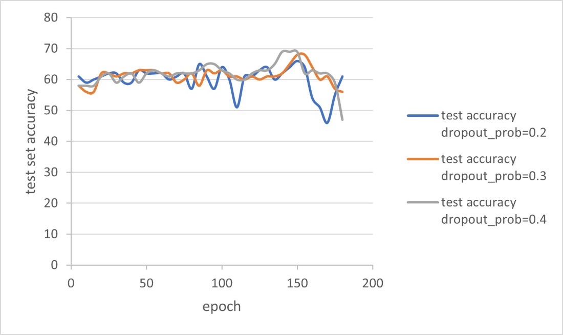
Figure 5: Trend of CNN’s accuracy (picture credit: original)

As shown in Figure 5, when the dropout probability is 0.2 to 0.4, the batch size is 64, and the learning rate is 0.0015, it is found that the recognition accuracy of basic CNN is about 66% to 69% after repeated training, and the highest accuracy is usually obtained at the 150th timestep. Due to the small number of samples in the test set, the accuracy obtained fluctuates greatly, but it still shows an overall upward trend in the first 150 timesteps.

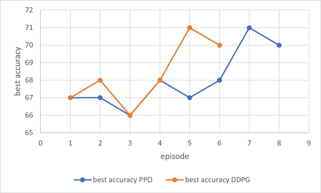
Figure 6: Trends of CNN’s accuracy after applying PPO/DDPG (picture credit: original)

As shown in Figure 6, both PPO and DDPG algorithms can effectively find the combination of hyperparameters that enable CNN model to obtain higher accuracy, and the result is about 71%. In addition, DDPG can use fewer timesteps to achieve the highest accuracy of CNN.

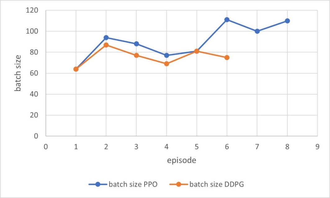
Figure 7: Trends of batch size after applying PPO/DDPG (picture credit: original)

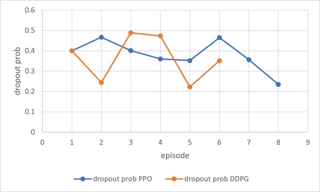
Figure 8: Trends of dropout prob after applying PPO/DDPG (picture credit: original)

According to Figure 7 and Figure 8, it can be seen that the agent has explored a variety of parameter combinations, and the final result shows that the batch size has been appropriately increased, while the dropout prob has been appropriately reduced, so that more information can be processed and more EEG signal features can be retained in a single iteration of deep learning. However, there are still potential risks such as overfitting. Table 2 shows the final results more clearly.

Table 2: Final result comparison

5. Conclusions

In this experiment, a new parameter adjustment method for deep learning is proposed, and the effectiveness of this method is verified based on the emotion classification problem, and the following conclusions are drawn. First, finding the optimal parameters through reinforcement learning methods such as PPO and DDPG effectively solves the problem of lengthy time and large amount of computational power in ordinary optimization. Second, the optimal accuracy of the CNN model in the experiment is about 71%. Third, compared with PPO, DDPG may converge to the best result faster.

Because the CNN model in this experiment receives relatively few parameter values, that is, the action vector dimension generated by the agent is low, which is not suitable for more complex networks and tasks. In the future, this method needs to be tested on more models and data sets. In addition, we should also explore the optimization method of generating higher dimensional motion vectors through agents, which may require more improvements to the current reward mechanism, or try more reinforcement learning algorithms. Finally, the improvement methods include but are not limited to: modifying the split ratio of the data set, increasing the timesteps of deep learning, increasing the number of training episodes of reinforcement learning, and dynamically adjusting the learning rate of reinforcement learning by using the cosine annealing learning rate. Thus, the method proposed in this paper has a huge development space, and also has a great help to improve the efficiency of deep learning.

References

[1]. Kanagaluru, V., & Sasikala, M. (2024). Two class motor imagery EEG signal classification for BCI using LDA and SVM. Traitement du Signal, 41(5).
[2]. Geng, Y., Shi, S., & Hao, X. (2024). Deep learning-based EEG emotion recognition: A comprehensive review. Neural Computing and Applications, 37(4), 1–32.
[3]. Zhao, Q., Zhao, D., & Yin, W. (2024). EEG emotion recognition based on GADF and AMB‐CNN model. International Journal of Numerical Modelling: Electronic Networks, Devices and Fields, 37(6).
[4]. Guo, L., Li, N., & Zhang, T. (2024). EEG-based emotion recognition via improved evolutionary convolutional neural network. International Journal of Bio-Inspired Computation, 23(4), 203–213.
[5]. Li, R., Yang, X., Lou, J., & others. (2024). A temporal-spectral graph convolutional neural network model for EEG emotion recognition within and across subjects. Brain Informatics, 11(1), 30.
[6]. Xu, B., Zhang, X., Zhang, X., & others. (2024). An improved graph convolutional neural network for EEG emotion recognition. Neural Computing and Applications, 36(36), 1–12.
[7]. Chen, W., Liao, Y., Dai, R., & others. (2024). EEG-based emotion recognition using graph convolutional neural network with dual attention mechanism. Frontiers in Computational Neuroscience, 18, 1416494.
[8]. Oka, H., Ono, K., & Panagiotis, A. (2024). Attention-based PSO-LSTM for emotion estimation using EEG. Sensors, 24(24), 8174.
[9]. Cunhang, F., Heng, X., Jianhua, T., & others. (2024). ICaps-ResLSTM: Improved capsule network and residual LSTM for EEG emotion recognition. Biomedical Signal Processing and Control, 87(PB).
[10]. Wang, S., Zhang, X., & Zhao, R. (2025). Lightweight CNN-CBAM-BiLSTM EEG emotion recognition based on multiband DE features. Biomedical Signal Processing and Control, 103, 107435.
[11]. Teng, W., Huang, X., Xiao, Z., & others. (2024). EEG emotion recognition based on differential entropy feature matrix through 2D-CNN-LSTM network. EURASIP Journal on Advances in Signal Processing, 2024(1).
[12]. Xueqing, L., Penghai, L., Zhendong, F., & others. (2023). Research on EEG emotion recognition based on CNN+BiLSTM+self-attention model. Optoelectronics Letters, 19(8), 506–512.
[13]. Koelstra, S., Mühl, C., & others. (2012). DEAP: A database for emotion analysis using physiological signals. IEEE Transactions on Affective Computing, 3(1), 18–31.
[14]. Vujji, A., Pusarla, N., Singh, A., & others. (2025). Emotion recognition using VMD domain bandwidth and spectral features. International Journal of Information Technology, (prepublish), 1–9.
[15]. Claudia, B., Andéol, C., Takuya, M., & others. (2023). Optimization of phase prediction for brain-state dependent stimulation: A grid-search approach. Journal of Neural Engineering, 20(1).
Cite this article
Mao,Y. (2025). Emotion Recognition Method Based on EEG Signal Reinforcement Learning and CNN. Applied and Computational Engineering,158,49-58.
Data availability
The datasets used and/or analyzed during the current study will be available from the authors upon reasonable request.
Disclaimer/Publisher's Note
The statements, opinions and data contained in all publications are solely those of the individual author(s) and contributor(s) and not of EWA Publishing and/or the editor(s). EWA Publishing and/or the editor(s) disclaim responsibility for any injury to people or property resulting from any ideas, methods, instructions or products referred to in the content.
About volume
Volume title: Proceedings of CONF-SEML 2025 Symposium: Machine Learning Theory and Applications
© 2024 by the author(s). Licensee EWA Publishing, Oxford, UK. This article is an open access article distributed under the terms and
conditions of the Creative Commons Attribution (CC BY) license. Authors who
publish this series agree to the following terms:
1. Authors retain copyright and grant the series right of first publication with the work simultaneously licensed under a Creative Commons
Attribution License that allows others to share the work with an acknowledgment of the work's authorship and initial publication in this
series.
2. Authors are able to enter into separate, additional contractual arrangements for the non-exclusive distribution of the series's published
version of the work (e.g., post it to an institutional repository or publish it in a book), with an acknowledgment of its initial
publication in this series.
3. Authors are permitted and encouraged to post their work online (e.g., in institutional repositories or on their website) prior to and
during the submission process, as it can lead to productive exchanges, as well as earlier and greater citation of published work (See
Open access policy for details).