1. Introduction

AMR technology empowers receiving devices to identify the modulation mode of unknown received signals in non-cooperative communication environments, and it holds significant application value in the field of wireless communication [1]. Additionally, Automatic Modulation Recognition (AMR) technology is pivotal in both military and civilian communication domains, playing a crucial role in various areas such as spectrum monitoring, cognitive radio, and signal control [2-3].

In recent years, considering the flexibility of deep learning multi-layer neural nonlinear transformation processing and various neural network concatenation methods, more and more deep learning based automatic modulation recognition model cameras have emerged. Throughout 2024, lightweight ICTNeT models based on convolutional neural networks and transformers, hybrid neural network models based on singular value decomposition, convolutional neural networks, and SE modules, as well as low signal-to-noise ratio models based on residual networks and transformers, have emerged successively [4-6].

Overall, the previously proposed automatic modulation recognition models have simulated large datasets in a specific signal-to-noise ratio environment and achieved a certain level of recognition accuracy and modulation speed. However, various types of networks can only achieve a certain outstanding function locally, and rarely can they achieve high recognition rates across different signal-to-noise ratio environments or maintain high recognition speeds while achieving considerable recognition rates.

In response to the aforementioned issues, this study proposes a fusion decision-making scheme based on convolutional neural networks, residual networks, and attention mechanisms, building upon previous experiments. In low signal-to-noise ratio environments, it aims to achieve high recognition rates while also ensuring a certain level of operating speed. To verify the accuracy of the established model in modulation recognition, this experiment chose to validate it on the DeepSig RadioML 2018.01A public dataset.

2. Model preparation

2.1. CNN

The diagram depicting the architecture of the convolutional neural network is presented in Figure 1.

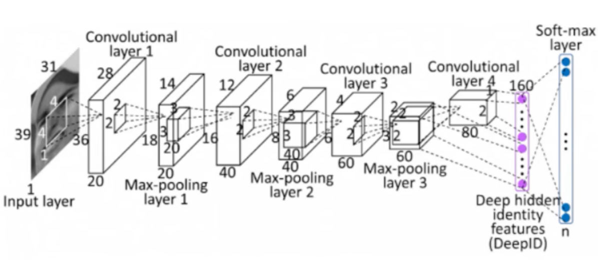
Figure 1: Convolutional neural network structure diagram

CNN, a feedforward neural network that integrates convolutional computation, has a deep architecture and is one of the key algorithms in deep learning [7-8]. It is built upon the visual perception mechanism of living organisms and can execute both supervised and unsupervised learning tasks. CNN is primarily made up of an input layer, a convolutional layer, a pooling layer, a fully connected layer, and an output layer.

The convolutional layer is responsible for extracting features from the input data, which includes several convolutional kernels. Each element of a convolutional kernel corresponds to a weight coefficient and a bias, similar to a neuron in a feedforward neural network. While operating, the convolutional kernels scan the input features in a systematic manner. They carry out matrix element multiplication and summation on the input features within the receptive field, followed by the addition of the bias value.

Taking two-dimensional convolution kernels as an instance:

\( {Z^{l+1}} \) (i,j)=[ \( {Z^{l}} ⊗{ω^{l+1}} \) ](i,j)+b=

\( \sum _{k=1}^{{K_{i}}}\sum _{x=1}^{f}\sum _{y=1}^{f}[Z_{k}^{l}({s_{0}}i+x,{s_{0}}j+y)ω_{k}^{l+1} \) (x,y)]+b (1)

(i,j) \( ∈ \) {0,1,..., \( {L_{l+1}} \) } \( {L_{l+1}} \) = \( \frac{{L_{l}}+2p-f}{{s_{0}}} \) +1

b represents the bias vector; \( { Z^{l+1}} \) and \( {Z^{l}} \) are the convolutional input and output of the layer respectively, also known as the feature map; \( {L_{l+1}} \) is the size of \( {Z^{l+1}} \) , assuming that the feature maps have the same length and width; Z(i,j) corresponds to the pixels of the feature map; K is the number of channels in the feature map; f, \( {s_{0}} \) and p are convolution layer parameters, corresponding to the size of the convolution kernel, stride, and padding layers. The schematic diagram of two-dimensional convolution is shown in Figure 2.

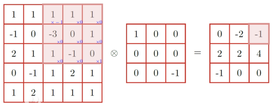
Figure 2: Example of two dimensional convolution

Once the feature extraction process is completed in the convolutional layer, the resultant feature map is forwarded to the pooling layer. The pooling layer proceeds to select and refine features from the feature map by substituting the values of individual points with statistical measures from their surrounding areas. Following this, the fully connected layer integrates the selected features in a nonlinear fashion to produce an output that is subsequently sent to the output layer. The output layer then utilizes logic or normalization functions to derive the ultimate classification labels.

2.2. ResNet

Despite the advantages of CNNs in feature extraction, as the depth of the network increases, training can become unstable and convergence slow. Additionally, during backpropagation, the gradients may diminish, leading to the vanishing gradient problem and significantly complicating the training process. Consequently, this study opts to incorporate residual networks into the architecture of convolutional neural networks, utilizing ResNet's residual blocks to address the "gradient vanishing" and "degradation problems" inherent in deep network learning.

ResNet, a convolutional neural network introduced by four researchers from Microsoft Research [9], employs internal residual blocks that bypass one or more layers via skip connections. This allows data from one layer to be directly passed to subsequent layers, thereby mitigating several issues associated with traditional deep CNNs. The schematic of the residual network link is depicted in Figure 3.

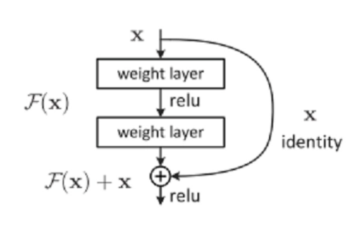
Figure 3: Schematic representation of a residual network connection

Assuming the mapping in the original deep network is H (x), in ResNet, this mapping is represented as the residual function F (x) plus the direct skip connection of the input x:

H(x)=F(x)+x (2)

Among them:

• x represents the input;

• F (x) represents the residual function to be learned, representing the change in input for a certain layer

2.3. Attention mechanism (SE module)

To enhance the network's representation capability, this study incorporated a channel attention mechanism. The concept of channel attention was introduced by Hu et al., and the core principle of SE is to adaptively recalibrate the feature responses of channel patterns by explicitly modeling the interdependence between channels [10]. The schematic representation of the channel attention mechanism is illustrated in Figure 4.

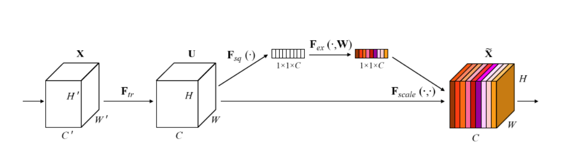
Figure 4: Schematic diagram of channel attention mechanism

The SE module is mainly completed by the following three operations:

(1) Squeeze ( \( {F_{sq}} \) ): This segment is tasked with globally averaging and pooling the feature maps to produce a vector of size 1*1*C, with each channel being denoted by a numerical value:

\( {z_{c}} \) = \( {F_{sq}} \) ( \( {u_{c}} \) )= \( \frac{1}{H*W}\sum _{i=1}^{H}\sum _{j=1}^{W}{u_{c}}(i.j) \) (3)

(2) Excitation ( \( {F_{ex}} \) ): This segment is finalized by two fully connected layers, which acquire the necessary weight information via the learned weights W, and eventually exhibit the required feature correlation:

s= \( {F_{ex}} \) (z,W)= \( σ \) (g(z,W))= \( σ \) ( \( {W_{2}}δ \) ( \( {W_{1}} \) z)) (4)

( \( {W_{1}} \) and \( {W_{2}} \) are two fully connected layers respectively.)

(1) Scale ( \( {F_{scale}} \) ): This section assigns weights to feature map U using the weight vector s generated in the second step, resulting in the desired feature map \( \widetilde{X} \) , which has the same size as feature map U:

\( \widetilde{{x_{c}}} \) = \( {F_{scale}} \) ( \( {u_{c}} \) , \( {s_{c}} \) )= \( {s_{c}}{u_{c}} \) (5)

After combining the channel attention mechanism, the model can enhance feature expression ability while maintaining computational efficiency and model simplicity.

3. Experimental description

3.1. Dataset and experimental environment settings

To accurately evaluate the performance of various AMR models in the experiment, this study selected the DeepSig RadioML 2018.01A dataset. The DeepSig RadioML 2018.01A dataset is an open-source dataset, widely utilized for wireless communication signal recognition, and was released by DeepSig Inc. [11]. It comprises signal samples from various modulation schemes at varying signal-to-noise ratios, making it suitable for training and evaluating both deep learning and machine learning algorithms. The configuration parameters of the DeepSig RadioML 2018.01A dataset are detailed in Table 1.

Table 1: DeepSig RadioML 2018.01A dataset

The dataset is segmented into a training set, a validation set, and a testing set for this experiment, with each set comprising 60%, 20%, and 20% of the data respectively. The experiment leverages the Keras 2.10.0 deep learning framework and operates with the Adam optimizer on an Intel (R) UHD Graphics environment.

3.2. Comparative experimental setup

In order to obtain more ideal experimental results, a total of three models were established in this experiment. The first is the basic CNN model, the second is the ReCNN model that combines CNN and ResNet, and the third is the new CNN_ResNet model that introduces channel attention mechanism in ResNet. Train three models in experimental environments with SNR of 0dB, 4dB, 10dB, 14dB, and 20dB, and obtain the final confusion matrix and recognition rate.

(1) CNN model: This model progressively uncovers the characteristics of input data by layering convolutional, pooling, Dropout, and fully connected layers, culminating in a classification prediction.The network architecture diagram of the CNN model is depicted in Figure 5.

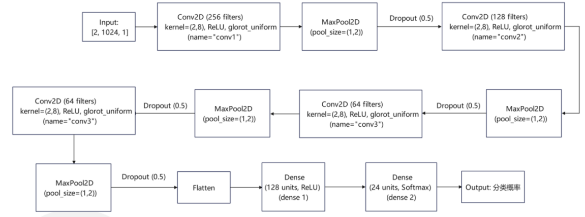
Figure 5: Diagram of the CNN model's network structure

(2) ReCNN model: This model incorporates a residual block following the convolutional block, which directly adds the input to the output via shortcut connections, thus facilitating the training of deeper networks. The diagram illustrating the network structure of the ReCNN model is shown in Figure 6.

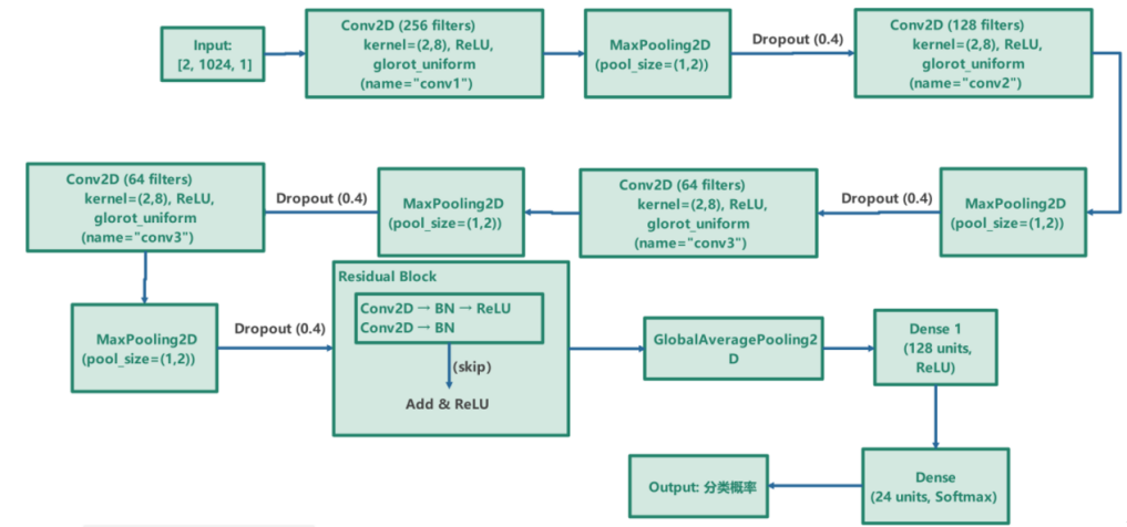
Figure 6: Network architecture diagram of ReCNN model

(3) CNN_ResNet model: This model defines a new Swish activation function to replace the original ReLU activation function, improving the performance of the model. Meanwhile, this model incorporates channel attention mechanism on the basis of residual blocks and replaces the original convolutional layers with separable convolutional layers. In order to achieve better convergence speed while ensuring a certain recognition rate, this experiment adjusted the proportion of convolutional layers and residuals in the original model to obtain better experimental results. The schematic diagram of the residual network structure combined with channel attention mechanism is shown in Figure 7. The diagram depicting the network structure of the CNN_ResNet model is displayed in Figure 8.

Figure 7: ResNet with SE module schematic diagram

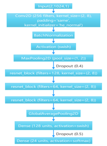
Figure 8: Network architecture diagram of CNN_ResNet model

3.3. Experimental results

Train the three models mentioned above in experimental settings with signal-to-noise ratios (SNRs) of 0dB, 4dB, 10dB, 14dB, and 20dB using the DeepSig RadioML 2018.01A dataset, and obtain the resultant recognition rates. The recognition rates of the various models across different SNR environments are presented in Table 2.

Table 2: Recognition rates of different models in different SNR environments

The line chart comparing the accuracy of different models in different SNR environments is shown in Figure 9.

Figure 9: Comparison of recognition rates of different models in different SNR environments

From the graph, it can be seen that the recognition rates of the CNN model in different SNR environments are 53.20%, 62.10%, 72.80%, 76.90%, and 77.00%, respectively. The recognition rates of the ReCNN model are 55.70%, 70.30%, 78.70%, 77.50%, and 68.20%. Compared to the original basic CNN model, the ReCNN model transformed 2.50%, 8.20%, 5.90%, 0.60%, and -8.80% in different SNR environments. The CNN_ResNet model showed significant improvements of 6.58%, 20.07%, 20.07%, 6.42%, and 2.01% compared to the CNN model in different SNR environments. It is evident from the experimental data that the ReCNN model only improves the recognition rate of the model in certain SNR environments, but the results are not satisfactory. The CNN_ResNet model showed good improvement in the final recognition rate under the SNR environment set in the experiment, and the effect was most significant in the SNR environments of 4dB and 10dB. The confusion matrix of the CNN_ResNet model under different SNR environments is shown in Figure 10.

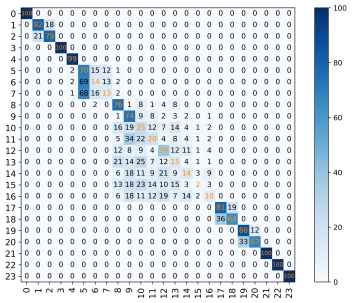
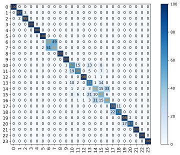
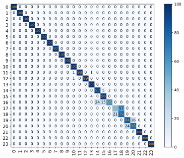
(a)SNR=0dB (b)SNR=4dB (c)SNR=10dB

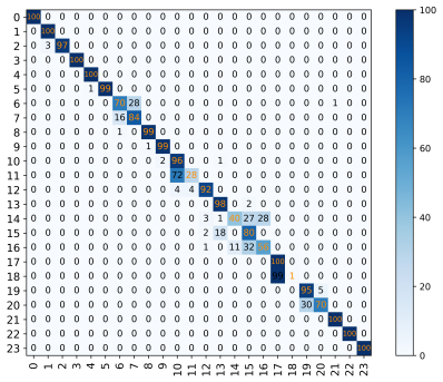
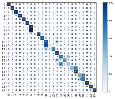
(d)SNR=14dB (e)SNR=20dB

Figure 10: The confusion matrix of CNN_ResNet model in different SNR environments

4. Conclusion

This experiment proposes a neural network model based on CNN, ResNet and SE module to address the problem of automatic modulation recognition being unable to achieve high recognition rates while maintaining a certain training speed in complex environments. This experiment established a total of three models, all of which were trained on the DeepSig RadioML 2018.01A dataset. Through comparative experiments, it was found that the CNN_ResNet model outperformed the other two models in terms of performance. This model can even achieve an accuracy of over 92% in an SNR=10dB environment and maintain an accuracy of around 60% in an SNR=0dB environment. However, the improvement in accuracy of the model has decreased in both high and low SNR environments. In future research, the model can be further optimized to adapt to more complex SNR environments.

References

[1]. Wu Changcheng, Sun Xiaochuan, Yu Jike, etc Lightweight modulation signal recognition method based on enhanced multi-scale feature fusion [J/OL]. Telecommunications Technology, 1-10 [2020-03-24] https://doi.org/10.20079/j.issn.1001-893x.240613002.
[2]. Gong An, Zhang Guilin, Mou Weiqing, etc Automatic modulation recognition method based on multi-layer wavelet decomposition convolutional neural network [J/OL]. Radio Communication Technology, 1-10 [2020-03-24] http://kns.cnki.net/kcms/detail/13.1099.TN.20241125.1432.004.html.
[3]. Zhou Shunyong, Lu Huan, Hu Qin, etc Automatic Modulation Recognition Based on SVD and Hybrid Neural Network Model [J]. Electronic Measurement Technology, 2024, 47 (21): 111-121. DOI: 10.19651/j.cnki-emt.2416437
[4]. Ma Wenxuan, Cai Zhuoran, Wang Chuan, etc Edge Device Modulation Recognition Method Based on Lightweight Hybrid Neural Network [J]. Information Adversarial Technology, 2024, 3 (06): 83-94
[5]. Zhou Shunyong, Lu Huan, Hu Qin, etc Automatic Modulation Recognition Based on SVD and Hybrid Neural Network Model [J]. Electronic Measurement Technology, 2024, 47 (21): 111-121. DOI: 10.19651/j.cnki-emt.2416437
[6]. Shen Danyang, Mai Wen Automatic modulation recognition of communication signals based on ResNet Transformer [J/OL]. Computer Engineering, 1-12 [2020-03-24] https://doi.org/10.19678/j.issn.1000-3428.0069677.
[7]. Goodfellow, I., Bengio, Y., Courville, A.·Deep learning (Vol. 1)·Cambridge:MIT press,2016
[8]. Gu, J., Wang, Z., Kuen, J., Ma, L., Shahroudy, A., Shuai, B., Liu, T., Wang, X., Wang, L., Wang, G. and Cai, J., 2015. Recent advances in convolutional neural networks. arXiv preprint arXiv:1512.07108.
[9]. He, K., Zhang, X., Ren, S. and Sun, J., 2016. Deep residual learning for image recognition. In Proceedings of the IEEE conference on computer vision and pattern recognition (pp. 770-778).
[10]. Hu J, Shen L, Sun G. Squeeze-and-Excitation Networks[C]//2018 IEEE/CVF Conference on Computer Vision and Pattern Recognition. Salt Lake City, UT, USA: IEEE, 2018: 7132-7141.
[11]. O’Shea T J, Roy T, Clancy T C. Over-the-Air Deep Learning Based Radio Signal Classification[J]. IEEE Journal of Selected Topics in Signal Processing, 2018, 12(1): 168-179.
Cite this article
Li,W. (2025). Automatic Modulation Recognition based on SE Module and CNN_ResNet. Applied and Computational Engineering,160,7-15.
Data availability
The datasets used and/or analyzed during the current study will be available from the authors upon reasonable request.
Disclaimer/Publisher's Note
The statements, opinions and data contained in all publications are solely those of the individual author(s) and contributor(s) and not of EWA Publishing and/or the editor(s). EWA Publishing and/or the editor(s) disclaim responsibility for any injury to people or property resulting from any ideas, methods, instructions or products referred to in the content.
About volume
Volume title: Proceedings of CONF-SEML 2025 Symposium: Machine Learning Theory and Applications
© 2024 by the author(s). Licensee EWA Publishing, Oxford, UK. This article is an open access article distributed under the terms and
conditions of the Creative Commons Attribution (CC BY) license. Authors who
publish this series agree to the following terms:
1. Authors retain copyright and grant the series right of first publication with the work simultaneously licensed under a Creative Commons
Attribution License that allows others to share the work with an acknowledgment of the work's authorship and initial publication in this
series.
2. Authors are able to enter into separate, additional contractual arrangements for the non-exclusive distribution of the series's published
version of the work (e.g., post it to an institutional repository or publish it in a book), with an acknowledgment of its initial
publication in this series.
3. Authors are permitted and encouraged to post their work online (e.g., in institutional repositories or on their website) prior to and
during the submission process, as it can lead to productive exchanges, as well as earlier and greater citation of published work (See
Open access policy for details).