1. Introduction

Trajectory tracking control plays a vital role in autonomous driving, aiming to generate smooth and accurate control commands that enable vehicles to follow predefined paths or trajectories safely and reliably [1]. Existing control methods for autonomous vehicles can generally be categorized into two approaches: traditional hierarchical control strategies and emerging end-to-end learning-based methods.

Traditional methods typically adopt a two-loop control framework that decouples position and velocity control. Path tracking is often achieved through the coordinated optimization of longitudinal and lateral control [2]. To achieve high-precision tracking, it is essential to match discrete path points in real time and design control algorithms based on vehicle kinematic or dynamic models. Significant progress has been made in this area, including sliding mode control [3, 4], Lyapunov stability-based approaches [5-6], and LQR-LMI parameter optimization [7], which have improved control efficiency in low-speed scenarios. Moreover, linear quadratic programming [8, 9] and model predictive control (MPC) [10-13] have enhanced algorithm adaptability through optimal solution search and constraint handling. Further developments such as adaptive robust controllers [14] and dual-loop MPC-LQR strategies [15] have strengthened robustness against parameter uncertainties.

Despite these advances, traditional methods face two major limitations. First, they rely heavily on manual parameter tuning and predefined reference points, lacking the ability to adaptively perceive changes in path curvature. Second, they exhibit limited robustness in handling multi-modal environmental features, which often compromises control accuracy in complex driving scenarios.

To overcome these challenges, end-to-end learning-based control methods have gained increasing attention. These methods employ deep learning architectures to directly map raw sensor inputs (e.g., camera images, LiDAR point clouds) to vehicle control commands (steering, throttle, brake), eliminating the need for complex intermediate modules such as perception, planning, and decision-making. Representative models include the CNN-based PilotNet and the CNN-LSTM model incorporating temporal dependencies. However, these methods still suffer from insufficient feature representation and limited capability in modeling long-term temporal dependencies.

Recently, Transformer models have shown great potential in autonomous driving, owing to their powerful self-attention mechanisms and capability to model complex dependencies. In perception tasks, Vision Transformers (ViT) extract global contextual features through patch-based image encoding, overcoming the local receptive field limitations of CNNs. In multi-modal fusion, cross-attention mechanisms enable the dynamic alignment of visual features and vehicle states (e.g., speed, acceleration), enhancing the sensitivity to critical information. Additionally, the Transformer-Decoder architecture supports autoregressive multi-step prediction, making it suitable for long-horizon control tasks.Existing studies have demonstrated that Transformer-based control models outperform traditional methods in terms of control accuracy (reducing MSE by 30%-50%), robustness in extreme scenarios (reducing collision rates to 4.2%), and interpretability (through attention visualization), highlighting their promising application prospects.

Nevertheless, the application of Transformer models in autonomous driving control remains at an early stage. Existing studies still face challenges such as limited feature fusion strategies, insufficient generalization of control policies, and a need for improved modeling of temporal dependencies and multi-modal perception capabilities.

To address these limitations, this paper proposes a Transformer-based end-to-end control model for autonomous driving. By leveraging self-attention mechanisms, the model enables dynamic fusion of multi-modal features and efficient modeling of long-term temporal dependencies. The proposed approach aims to overcome the reliance on local path information in traditional algorithms and improve control accuracy, robustness, and interpretability in dynamic driving environments.

The main contributions of this paper are summarized as follows.

(1) This paper designs an end-to-end Transformer control architecture consisting of input encoding, multi-modal feature fusion, and control signal decoding to address the challenges of multi-modal fusion and temporal dependency modeling.

(2) This paper proposes a cross-attention-based feature fusion strategy to effectively align and complement visual features and vehicle states.

(3) This paper constructs a multi-scenario autonomous driving dataset using the CARLA simulation platform and evaluates the proposed model in terms of control accuracy, driving safety, real-time performance, robustness, and interpretability.

(4) This paper analyzes the impact of multi-frame temporal inputs, an 8-head attention mechanism, and cross-attention fusion strategies on model performance, demonstrating the practical potential and competitiveness of the proposed approach.

2. Methodology

2.1. Model architecture

The input encoding module extracts features from visual and vehicle state information. For visual feature extraction, this paper adopt the Vision Transformer (ViT-B/16) as the backbone. Each image frame is divided into a sequence of patches, which are then processed by a 12-layer Transformer encoder to capture global contextual information. To handle temporal dependencies, features from multiple consecutive frames are independently encoded and concatenated along the temporal axis. The vehicle state encoder processes either a 4-dimensional vector (current speed and three-axis acceleration) or a 20-dimensional sequence vector (historical data from the past 5 frames). The input is projected into a 256-dimensional embedding through stacked fully connected layers. If the dimensionality of the visual features differs, an additional projection layer aligns them to the same 256 dimensions, ensuring compatibility for subsequent fusion.

The multi-modal fusion module concatenates the visual feature sequence with the vehicle state token, forming a unified input sequence. For instance, with 5 input image frames, the visual features form a sequence of 985×768, which is concatenated with a 1×768 vehicle state token to create a combined sequence of 986×768. To preserve structural information, there are three types of positional encodings. First of all, Temporal Positional Encoding is introduced to distinguish the sequence order of multiple frames. In addition, Spatial Positional Encoding, inherited from the original ViT patch positions, is used to retain spatial relationships within each frame. Lastly, Modality Type Encoding is specifically added to the vehicle state token in order to differentiate between visual and non-visual modalities. The vehicle state token is independently encoded to prevent interference with visual features while enabling effective fusion through attention mechanisms.

A lightweight regression head utilizes the first token of the fused sequence (either the CLS token or vehicle state token) as the global context. The output is passed through stacked fully connected layers to regress three control commands: steering angle, throttle, and brake. Specifically, the steering angle output is constrained within the range of [-1, 1] using the Tanh activation function, while throttle and brake values are limited to [0, 1] using the Sigmoid activation function. Optionally, for tasks requiring multi-step future control prediction, a Transformer Decoder with three layers and eight attention heads is employed. The decoder adopts an autoregressive strategy, using teacher forcing during training and iterative generation during inference. The input consists of the encoder’s fused features and embedded historical control signals, and the output is a 3×3-dimensional prediction of future control commands over the next three steps.

2.2. Training strategy

2.2.1. Loss function

This paper uses Mean Squared Error (MSE) loss as the primary objective to regress continuous control signals (steering angle, throttle, and brake). For discrete control actions, such as throttle/brake classification, Cross-Entropy (CE) loss is optionally applied.

The MSE loss is defined as:

\( {L_{MSE}}=\frac{1}{N}\sum _{i=1}^{N} \sum _{j=1}^{3} {({y_{i,j}}-{\hat{y}_{i,j}})^{2}}\ \ \ (1) \)

The CE loss is defined as:

\( {L_{CE}}=-\frac{1}{N}\sum _{i=1}^{N} \sum _{c=1}^{C} {y_{i,c}}log{({\hat{y}_{i,c}})}\ \ \ (2) \)

The total loss is a weighted combination:

\( {L_{total}}=α{L_{MSE}}+(1-α){L_{CE}}\ \ \ (3) \)

Where α is a balancing coefficient.

3. Experimental setup

3.1. Dataset and data collection

The dataset used in this study was collected from the CARLA simulator, which provides diverse synthetic data under various weather and lighting conditions. The dataset covers multiple driving scenarios, including urban roads (Town01), complex intersections (Town03), and highways (Town07). It incorporates a wide range of environmental settings, such as different weather conditions (clear, rain, fog, snow) and lighting variations (noon, dusk, night). In addition, traffic density is categorized into three levels: low, medium, and high. The driving tasks include lane-keeping, turning, lane-changing, emergency obstacle avoidance, and intersection handling. The sensor configuration consists of a front-view RGB camera with a 90° field of view (FOV) and a resolution of 1920×1080, capturing images at 20 Hz. Simultaneously, vehicle states (speed, acceleration, steering angle) and control signals (steering angle, throttle, brake) are recorded at the same frequency. The dataset is stored in PNG image files for visual data and JSON files for vehicle states and control signals, with each file labeled by a timestamp for synchronization and easy identification.

3.2. Data preprocessing

Data preprocessing involves image processing, data augmentation, vehicle state synchronization, and dataset partitioning. For image processing, all images are resized to 224×224 pixels and normalized to the [0, 1] range. A sequence of 5 consecutive frames (captured at 0.1-second intervals) is used as the model input to capture temporal dynamics. To enhance data diversity and improve model generalization, a series of advanced data augmentation techniques are employed. Firstly, stochastic adjustments to brightness and contrast are applied within a ±20% range to simulate varying lighting conditions. Secondly, synthetic motion blur is introduced using convolutional kernels ranging from 3×3 to 15×15, mimicking camera or object movement. Thirdly, Gaussian noise with a standard deviation (σ) between 0.01 and 0.05 is injected into the images to emulate sensor noise and improve robustness under noisy input conditions. For vehicle state synchronization, interpolation is utilized to ensure precise alignment between each image frame and its corresponding vehicle state data. Following this process, the dataset is partitioned into three distinct subsets. The training set, comprising 70 percent of the scenarios, encompasses the full spectrum of weather and lighting combinations to support comprehensive learning. The validation set, accounting for 15 percent of the scenarios, is restricted to daytime conditions under clear or rainy weather, serving to fine-tune model performance. The test set, also representing 15 percent of the scenarios, is reserved for evaluating the model under previously unseen extreme conditions, such as dense fog during nighttime, thereby assessing its generalization capability in challenging environments. A summary of the dataset partitioning is provided in Table 1.

Table 1: Description of dataset fields

3.3. Experimental environment

3.3.1. Hardware configuration

All experiments were conducted on a high-performance computing cluster equipped with 8 NVIDIA A100 GPUs, each with 80 GB of memory, supporting distributed training and mixed-precision computation. The server is powered by an Intel Xeon Platinum 8369B processor (64 cores, 128 threads, 2.7 GHz base frequency), accompanied by 512 GB DDR4 ECC memory (3200 MHz) and a 4 TB NVMe SSD (7 GB/s read/write speed) for high-speed data caching and storage of training logs. Additionally, the cluster utilizes an InfiniBand HDR interconnect with a bandwidth of 200 Gbps to support efficient multi-node and multi-GPU parallel training.

3.3.2. Software environment and framework

The system runs on Ubuntu 20.04 LTS (kernel version 5.15.0) and adopts PyTorch 2.0.1 as the deep learning framework, accelerated by CUDA 12.1 and cuDNN 8.9.6 libraries. The CARLA simulator (version 0.9.14) is used for automated multi-modal data collection through its Python API, synchronizing images (PNG format) and metadata (JSON format) on a per-frame basis. Additional software dependencies include: (1) NumPy and Pandas for data processing, (2) OpenCV for image enhancement and normalization, (3) NCCL and Apex for distributed training and mixed-precision computation, and (4) Matplotlib and TensorBoard for visualization. The development environment is based on Python 3.9.16, with package management handled by Conda. Version control is maintained using Git, and the entire system is containerized using Docker, with the base image provided by NVIDIA's NGC repository (nvcr.io/nvidia/pytorch:23.05-py3).

4. Experimental results and analysis

4.1. Control performance evaluation

4.1.1. Control accuracy

As shown in Table 2, the proposed Transformer-based model consistently outperforms both the CNN-LSTM and the Pure CNN (PilotNet) baselines in terms of control accuracy. Specifically, the Transformer model achieves a lower Mean Squared Error (MSE) for steering angle and throttle/brake prediction, as well as a smaller Mean Absolute Error (MAE) for overall control performance. These results demonstrate the superior capability of the Transformer architecture in capturing complex feature dependencies and generating more accurate control commands.

Table 2: Comparison of control accuracy

The proposed Transformer-based model achieves an MSE of 0.008 for steering angle, an MSE of 0.015 for throttle/brake prediction, and an overall MAE of 0.023. All these metrics are significantly lower than those of the CNN-LSTM and Pure CNN (PilotNet) baselines, indicating the superior control accuracy of the Transformer model.

4.1.2. Driving safety

As shown in Table 3, the proposed Transformer-based model demonstrates superior performance across three key safety metrics: collision rate, lane departure frequency, and average number of human interventions. In all cases, the Transformer model achieves significantly lower values compared to the CNN-LSTM and Pure CNN (PilotNet) baselines. Specifically, the model effectively reduces the risk of collisions, maintains better lane stability, and decreases the frequency of human interventions required to correct driving errors. These results confirm that the Transformer architecture not only improves control accuracy but also enhances overall driving safety in complex environments.

Table 3: Comparison of driving safety performance

4.1.3. Real-time performance

As shown in Table 4, all three models — Transformer (ViT), Transformer (ResNet), and Pure CNN (PilotNet) — meet the target requirement for single-frame inference time (≤50 ms). Notably, the Transformer (ResNet) and Pure CNN (PilotNet) models achieve particularly fast inference speeds of 25 ms and 22 ms per frame, respectively, which are significantly below the target threshold. These results indicate that both models offer strong potential for real-time autonomous driving applications.

Table 4: Comparison of real-time inference performance

4.2. Comparative experiments

4.2.1. Baseline model comparison

As shown in Table 5, the proposed Transformer-based model demonstrates outstanding overall performance across multiple evaluation metrics, including model size, control accuracy, driving safety, and real-time inference. Compared to the CNN-LSTM and Pure CNN (PilotNet) baselines, the Transformer model has a larger number of parameters. However, it achieves superior control accuracy and driving safety, with significantly lower MSE and collision rate. Moreover, the Transformer model maintains competitive real-time performance, with a single-frame inference time of only 40 ms, well within the target requirement. These results indicate that although the Transformer model increases model complexity, it offers substantial advantages in control precision and driving safety, while still satisfying the demands of real-time autonomous driving applications.

Table 5: Comparison of baseline models

4.2.2. Ablation study results

Table 6 presents the impact of multi-frame temporal input on model performance. Using a sequence of 5 consecutive frames significantly improves both control accuracy and driving safety compared to single-frame input. Specifically, the steering angle MSE decreases from 0.036 to 0.023, while the collision rate under rainy conditions drops from 9.1% to 4.2%. Although the inference time increases slightly from 35 ms to 40 ms, it remains within the acceptable real-time range. These results indicate that incorporating multi-frame temporal information enables the model to better capture driving patterns, leading to enhanced control precision and safety in autonomous driving tasks.

According to the analysis in Table 6, incorporating multi-frame temporal information (5 frames) significantly improves model performance compared to single-frame input. Specifically, the steering angle MSE is reduced from 0.036 to 0.023, while the collision rate under rainy conditions decreases from 9.1% to 4.2%. These improvements suggest that multi-frame inputs enable the model to better capture temporal dependencies and predict vehicle trajectories more accurately, thereby enhancing control precision and driving safety. Although the inference time slightly increases from 35 ms to 40 ms, it remains well within the acceptable range for real-time autonomous driving applications. Overall, the use of multi-frame temporal information proves to be an effective strategy for improving the performance and robustness of autonomous driving systems.

Table 6: Impact of multi-frame temporal input on model performance

Table 7 presents the impact of varying the number of attention heads on model performance. The results indicate that the number of attention heads affects both model accuracy and resource consumption. When using 8 attention heads, the model achieves the best overall performance, with the lowest MSE of 0.023. Additionally, GPU memory usage and training convergence steps remain within a reasonable range. In comparison, the 4-head configuration consumes the least GPU memory but suffers from higher MSE. On the other hand, increasing the number of attention heads to 16 leads to slightly better performance than 4 heads, but with a substantial increase in GPU memory consumption, and no significant reduction in training steps. Overall, these results suggest that selecting the appropriate number of attention heads requires balancing control accuracy, memory efficiency, and training cost. In this study, the 8-head configuration provides the most favorable trade-off.

Table 7: Impact of attention head numbers on model performance

Table 8 compares the performance of two different vehicle state fusion strategies: simple concatenation and cross-attention fusion. The results show that the cross-attention fusion strategy achieves better throttle control accuracy, with a lower MSE of 0.012 compared to 0.015 for the concatenation method. In addition, the cross-attention approach exhibits stronger robustness in extreme scenarios, with a smaller performance degradation (+8% vs. +15%), indicating its superior ability to adapt to complex environments. Furthermore, the cross-attention fusion strategy receives a higher interpretability score (4.5/5.0 vs. 3.2/5.0), suggesting that its attention weight allocation is more reasonable and easier to understand. Overall, these results demonstrate that the cross-attention fusion strategy provides better performance, robustness, and interpretability for integrating vehicle state information.

Table 8: Comparison of vehicle state fusion strategies

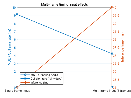
Figure 1: Impact of multi-frame temporal input (picture credit: original)

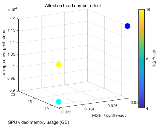
Figure 2: Optimization of attention head numbers (picture credit: original)

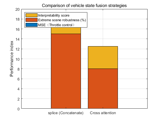
Figure 3: Comparison of vehicle state fusion strategies (picture credit: original)

All experiments were conducted on the CARLA simulation test set, with a particular focus on performance under extreme scenarios, such as dense fog combined with nighttime conditions. The evaluation metrics include: The increase in MAE under extreme scenarios compared to normal conditions, which reflects the degree of performance degradation (↑ indicates worse performance). The interpretability score, rated by domain experts on a 5-point scale, assesses the reasonableness of the attention weight distribution within the model (The relevant process studies and comparisons are shown in Figures 1, 2, and 3).

4.3. Robustness analysis

4.3.1. Impact of weather conditions on performance

Table 9 presents the comparison results of model performance under different weather conditions. The Transformer-based model consistently achieves lower MSE values than the CNN-LSTM and Pure CNN baselines across all weather scenarios, demonstrating superior robustness. Specifically, under clear weather conditions (baseline), the Transformer model achieves an MSE of only 0.023. As weather conditions deteriorate, such as in rainy or foggy environments, the MSE values of all models increase. However, the performance degradation of the Transformer model remains significantly smaller compared to the other two models, highlighting its stronger ability to cope with challenging environmental variations.

Table 9: Impact of weather conditions on model performance

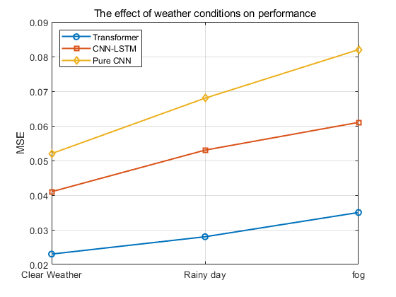
Figure 4: Comparison of model performance under different weather conditions (picture credit: original)

As shown in Figure 4, under rainy conditions, the MSE of the Transformer model increases by 21.7%, while the CNN-LSTM and Pure CNN models experience larger increases of 29.3% and 30.8%, respectively. In foggy conditions, although the MSE of the Transformer model increases by 52.2%, this degradation is still smaller than that of the CNN-LSTM (48.8%) and Pure CNN (57.7%) models. These results indicate that the Transformer model demonstrates stronger adaptability and robustness across varying weather conditions.

4.3.2. Performance degradation under lighting variations

Table 10 shows the performance comparison of different models under various lighting conditions. The Transformer model consistently achieves lower MSE values than the CNN-LSTM and Pure CNN baselines, demonstrating superior adaptability. Under daytime (baseline) conditions, the Transformer model achieves the lowest MSE of 0.023. As lighting conditions deteriorate — such as during dusk or nighttime — all models exhibit increased MSE values. However, the performance degradation of the Transformer model remains relatively small, confirming its robustness against lighting variations.

Table 10: Performance degradation under different lighting conditions

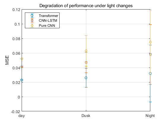
Figure 5: Performance degradation under different lighting conditions (picture credit: original)

As shown in Figure 5, under dusk conditions, the MSE of the Transformer model increases by 13.0%, while the CNN-LSTM and Pure CNN models experience larger increases of 14.6% and 21.2%, respectively. Under nighttime conditions, although the MSE of the Transformer model increases by 39.1%, this degradation remains smaller than that of CNN-LSTM (41.5%) and Pure CNN (44.2%). These results demonstrate that the Transformer model maintains better robustness and stability under varying lighting conditions, effectively reducing performance degradation in challenging visual environments.

4.4. Interpretability analysis

4.4.1. Attention weight visualization

The Transformer model, empowered by its self-attention mechanism, demonstrates a remarkable ability to capture long-range dependencies, making it particularly effective for autonomous driving control tasks. To further investigate the model's decision-making rationale, this paper conducted a comprehensive visualization analysis of the attention weights within the multi-modal fusion module.

Specifically, this paper extracted the attention weight matrices from the last layer of the Transformer Encoder in the visual feature encoder (e.g., ViT or ResNet). The attention scores of each image patch were calculated and aggregated across multiple consecutive frames to generate a dynamic heatmap sequence. This visualization intuitively illustrates the regions of interest that the model focuses on overtime during the driving process.

In addition, for the vehicle state encoder, this paper analyzed the weight distribution of the cross-attention module. The results highlight the critical role of vehicle state information (such as speed and acceleration) in influencing the final control signals, further demonstrating the interpretability of the proposed model's decision logic.

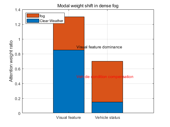
Figure 6: Shift of attention weights towards vehicle state information in foggy scenarios (picture credit: original)

In typical driving scenarios, the model's attention weights are highly concentrated on critical regions such as road boundaries, obstacle contours, and traffic lights. This indicates that the Transformer-based model effectively captures key visual cues to support accurate control decisions. However, under extreme weather conditions such as dense fog, where visual features become severely blurred, the model adapts by shifting its attention towards vehicle state information, such as acceleration changes, to compensate for the loss of visual cues. As shown in Figure 6, this dynamic adjustment highlights the model's ability to flexibly leverage multi-modal information, enhancing its robustness in complex and challenging environments.

4.4.2. Evaluation of decision logic consistency

To evaluate the consistency between the model's decision logic and human driving knowledge, both quantitative and qualitative methods were used. For the quantitative evaluation, a driving rule set was established to measure the rule compliance rate of model predictions. Results show that the Transformer model achieved a rule compliance rate of 92.3% in clear weather, outperforming CNN-LSTM (85.1%) and Pure CNN (78.6%). For the qualitative evaluation, five autonomous driving experts were invited to rate the model’s decisions in 100 extreme scenarios. The Transformer model received an average score of 4.2 (standard deviation 0.3) out of 5.0. Experts noted that its attention allocation is closely aligned with human-like visual-state coordination strategies, as illustrated in Figure 7.

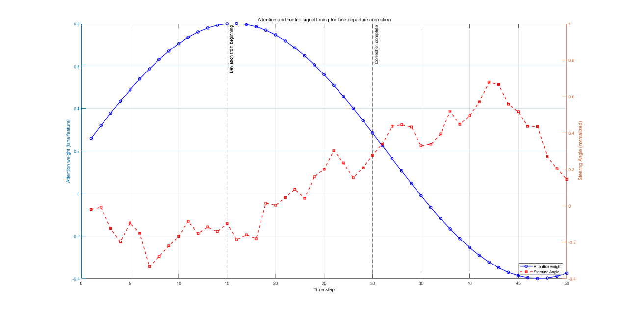
Figure 7: Temporal evolution of lane departure correction case (picture credit: original)

Case studies further demonstrate that in lane departure scenarios, the Transformer model increases attention to lane markings and promptly corrects the steering angle. In addition, SHAP analysis was applied to quantify the contribution of visual features and vehicle states to control outputs. The results show that visual features play a dominant role in steering angle prediction, while vehicle states are critical for throttle and brake control. Overall, the Transformer model achieves a human-like decision-making process by combining explicit attention mechanisms with implicit feature fusion, offering significantly better interpretability than traditional end-to-end models.

5. Conclusion

This paper presents a Transformer-based end-to-end control model for autonomous driving, addressing key limitations of traditional control approaches. The proposed model integrates input encoding, multi-modal fusion, and control signal decoding modules to enable effective fusion of multi-modal features and long-term temporal modeling. The training strategy combines MSE and cross-entropy loss functions, the AdamW optimizer, cosine annealing learning rate scheduling, and regularization techniques such as dropout and label smoothing. Experimental results demonstrate that the Transformer-based model outperforms CNN-LSTM and Pure CNN (PilotNet) baselines across multiple dimensions, including control accuracy, driving safety, real-time performance, robustness, and interpretability. In particular, the use of multi-frame temporal inputs, an 8-head attention mechanism, and cross-attention fusion strategies further enhance model performance. Overall, this study shows that the proposed Transformer-based end-to-end control model offers strong competitiveness and application potential, providing new insights for the development of autonomous driving technologies.

References

[1]. Paden, B., Čáp, M., Yong, S. Z., Yershov, D., & Frazzoli, E. (2016). A survey of motion planning and control techniques for self-driving urban vehicles. IEEE Transactions on Intelligent Vehicles, 1(1), 33–55.
[2]. Guldner, J., Utkin, V. I., & Ackermann, J. (1994). A sliding mode control approach to automatic car steering. In Proceedings of the 1994 American Control Conference (pp. 1969–1973). IEEE.
[3]. Guo, J., Luo, Y., & Li, K. (2017). An adaptive hierarchical trajectory following control approach of autonomous four-wheel independent drive electric vehicles. IEEE Transactions on Intelligent Transportation Systems, 18(10), 2825–2835.
[4]. Park, B. S., Yoo, S. J., Park, J. B., & Choi, Y. H. (2010). A simple adaptive control approach for trajectory tracking of electrically driven nonholonomic mobile robots. IEEE Transactions on Control Systems Technology, 18(5), 1199–1206.
[5]. Park, S., Deyst, J., & How, J. P. (2007). Performance and Lyapunov stability of a nonlinear path following guidance method. Journal of Guidance, Control, and Dynamics, 30(6), 1718–1728.
[6]. Alcalá, E., Puig, V., Quevedo, J., Escobet, T., & Comasolivas, R. (2018). Autonomous vehicle control using a kinematic Lyapunov-based technique with LQR-LMI tuning. Control Engineering Practice, 73, 1–12.
[7]. Li, Y., Wang, X. N., Li, S. J., & Zhu, J. (2014). LQR based trajectory tracking control for forked AGV. Applied Mechanics and Materials, 577, 447–451.
[8]. Liang, C. H., Liu, Y. H., & Wang, Y. (2021). Lateral control using LQR for intelligent vehicles based on the optimal front-tire lateral force. Journal of Tsinghua University (Science and Technology), 61(9), 906–912.
[9]. Tajaddini, N., Tajaddini, M., & Hashemi, R. (2015). An optimal integrated longitudinal and lateral dynamic controller development for vehicle path tracking. Latin American Journal of Solids and Structures, 12(6), 1006–1023.
[10]. Hu, C., Wang, R., Yan, F., & Chen, N. (2016). Output constraint control on path following of four-wheel independently actuated autonomous ground vehicles. IEEE Transactions on Vehicular Technology, 65(6), 4033–4043. https://doi.org/10.1109/TVT.2015.2452931
[11]. Fnadi, M., Du, W., Plumet, F., & Benamar, F. (2020). Constrained model predictive control for dynamic path tracking of a bi-steerable rover on slippery grounds. Control Engineering Practice, 107, 104693.
[12]. Ming, T., Deng, W., Zhang, S., & Zhu, B. (2016). MPC-based trajectory tracking control for intelligent vehicles. SAE Technical Paper, 2016-01-0452.
[13]. Falcone, P., Borrelli, F., Asgari, J., Tseng, H. E., & Hrovat, D. (2007). Predictive active steering control for autonomous vehicle systems. IEEE Transactions on Control Systems Technology, 15(3), 566–580.
[14]. Gu, D., & Hu, H. (2006). Receding horizon tracking control of wheeled mobile robots. IEEE Transactions on Control Systems Technology, 14(4), 743–749.
[15]. Alcalá, E., Puig, V., & Quevedo, J. (2019). TS-MPC for autonomous vehicles including a TS-MHE-UIO estimator. IEEE Transactions on Vehicular Technology, 68(2), 1153–1163.
Cite this article
Zhao,H. (2025). Research on Transformer Models for End-to-End Control in Autonomous Driving. Applied and Computational Engineering,160,210-222.
Data availability
The datasets used and/or analyzed during the current study will be available from the authors upon reasonable request.
Disclaimer/Publisher's Note
The statements, opinions and data contained in all publications are solely those of the individual author(s) and contributor(s) and not of EWA Publishing and/or the editor(s). EWA Publishing and/or the editor(s) disclaim responsibility for any injury to people or property resulting from any ideas, methods, instructions or products referred to in the content.
About volume
Volume title: Proceedings of CONF-SEML 2025 Symposium: Machine Learning Theory and Applications
© 2024 by the author(s). Licensee EWA Publishing, Oxford, UK. This article is an open access article distributed under the terms and
conditions of the Creative Commons Attribution (CC BY) license. Authors who
publish this series agree to the following terms:
1. Authors retain copyright and grant the series right of first publication with the work simultaneously licensed under a Creative Commons
Attribution License that allows others to share the work with an acknowledgment of the work's authorship and initial publication in this
series.
2. Authors are able to enter into separate, additional contractual arrangements for the non-exclusive distribution of the series's published
version of the work (e.g., post it to an institutional repository or publish it in a book), with an acknowledgment of its initial
publication in this series.
3. Authors are permitted and encouraged to post their work online (e.g., in institutional repositories or on their website) prior to and
during the submission process, as it can lead to productive exchanges, as well as earlier and greater citation of published work (See
Open access policy for details).