1.  Introduction

Due to long-term use and natural weathering, ancient architectural steps are often subject to uneven wear and tear, such as depressions in the center and scratches on the surface. In order to investigate the use and wear patterns of steps, the study centers on step wear and pedestrian flow, focusing on eight tasks: analyzing the frequency of use, the preference of pedestrian walking direction, the number of people using the steps at the same time and the walking pattern (side-by-side or sequential), evaluating the consistency of wear and tear with the existing information, deducing the age and reliability of the steps, tracing the history of maintenance, verifying the source of the materials, and the pattern of change of the flow of people in different time periods. These tasks aim to reveal the association between step wear, human activities, and material properties through multi-dimensional analysis to provide a basis for scientific maintenance.

In this study, an analytical model is constructed based on four assumptions: first, it is assumed that step wear increases uniformly with time under normal use, and the future state can be predicted by linear regression; second, 3D laser scanning is used to accurately obtain step surface data and quantify the depth and area of wear; third, it is assumed that the effects of pedestrian flow, frequency of use, and material on wear are independent of each other, which facilitates single-factor analysis; and finally, it is assumed that the data collected are comprehensive and accurate, which ensures the reliability of the model. collected data are comprehensive and accurate to ensure the reliability of the model. Through the analysis of thermal imaging and basic prediction map, it is initially verified that the degree of wear is positively correlated with natural and human factors, which lays the foundation for the subsequent establishment of a scientific wear prediction and maintenance decision-making model.

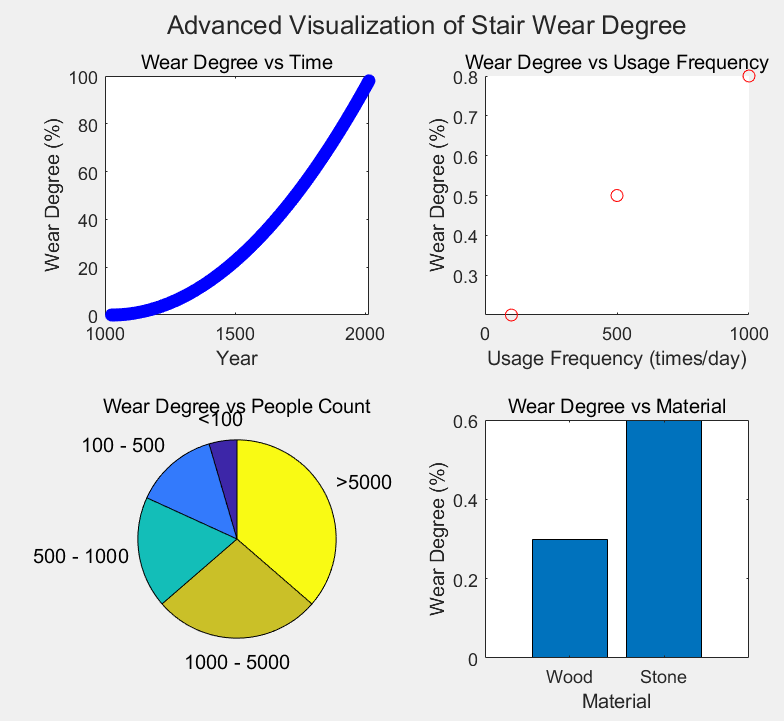
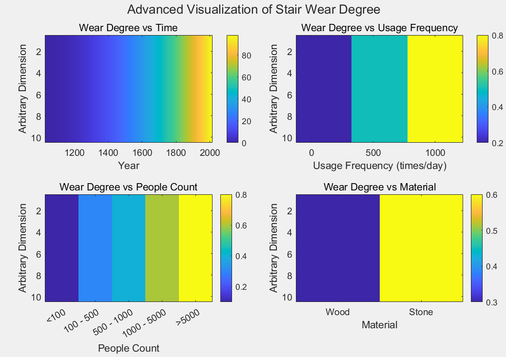
The following figure 1 shows the basic predictions of the varying degrees of wear with different factors. We first presented different types of basic images for analysis. For further research, we then used thermal imaging to visually display the effect of the changes.The results are shown in Figure 1.

2.  Model building

2.1.  Model I: Wear model of stairs in ancient buildings

Historical research shows that regardless of the durability of the materials, all structures wear out over time due to the continuous action of external forces [1]. Ancient staircases were necessary for connecting floors and supporting foot traffic, and they would experience friction and pressure during daily use. Uneven walking patterns and different usage frequencies led to uneven wear. For instance, in many temples and churches, the centers of the steps wore out more than the edges due to frequent trampling, causing the originally flat surfaces to become curved.

To study this kind of wear, we used a laser rangefinder for precise depth measurement, digital image analysis for wear distribution, and 3D scanning for detailed model analysis. By modeling factors such as usage frequency, walking direction, and concurrent users, and analyzing wear data across time and regions, we established a mathematical model that accurately reflects the actual usage and wear patterns of the stairs.

Based on the description just provided, we innovatively set wear as a quantifiable indicator, wear degree d(x,y), expressed as a percentage coefficient. Then, through the analysis of the initial wear data, the wear degree is set to be mainly affected by the wear depth d₁(x,y), while also being influenced by secondary conditions such as surface flatness d₂, scratches d₃, and dents d₄. Therefore, the wear degree d(x,y) can be calculated as follows:

Among them, w₁, w₂, w₃, and w₄ are the influence weight coefficients of the wear depth d₁(x,y), surface flatness d₂, scratch d₃, and dent d₄ on the wear degree d(x,y), respectively. The determination of these weight coefficients should be based on specific research purposes and actual conditions, and set through experimental data or empirical judgment. Our research focus is on the macroscopic wear changes on the surface, that is, a larger weight w₁ is assigned to the wear depth d₁(x,y).

After further quantifying the wear as the wear depth d₁(x,y), we can conduct a data-based analysis of the wear and find that it is related to factors such as the material's wear resistance coefficient, usage frequency, directional relationship, and the number of users. Through further design, the wear depth d₁(x,y) can be calculated by the following method:

Among them, a is the wear resistance coefficient of the material ; f(x,y) represents the usage frequency ; v(x, y) represents the relation of direction ; n(x, y) represents the number of users ; e(x, y) is the error term.

This formula establishes a quantitative relationship between wear depth d₁(x,y), usage frequency f(x,y), directional relationship v(x,y), and material property a. It allows us to analyze the impact of these factors on wear depth. For example, with other factors constant, higher usage frequency f(x,y) leads to greater wear depth d₁(x,y). Including the error term e(x,y) makes the model more realistic, as actual wear is influenced by multiple complex factors. This formula provides a foundation for studying stair wear mechanisms and inferring stair usage from measured wear depth.

To analyze the staircase wear data, we focus on three key factors: usage frequency f(x,y), directional relationship n(x,y), and error term e(x,y). Usage frequency f(x,y) depends on the building's function, usage time, and foot traffic. For instance, temple staircases see higher usage during religious festivals, while residential staircases have stable but fluctuating patterns, especially during peak hours like mornings and evenings. We approximate f(x,y) as the number of people passing a specific point (x,y) within a time period T.

This formula provides an intuitive method for quantifying usage frequency, which is crucial for studying the wear patterns of stairs, as usage frequency is one of the key factors influencing the depth of wear. By analyzing the distribution of usage frequency at different positions on the stairs, we can further understand the reasons for the differences in wear in different areas of the stairs.

The directional relationship v(x,y) reflects people's walking preferences on stairs, influenced by factors like stair layout, building function, and walking habits. For example, if a staircase connects an entrance hall with office floors, people may predominantly walk upwards in the morning and downwards in the evening. Additionally, physical factors such as stair width and handrail position can also affect walking direction.

We can define a directional preference coefficient to quantify the directional relationship. Suppose within a certain time period, the number of people passing through the staircase position (x, y) in a certain direction (such as the upward direction) is N_up(x, y), and the number of people passing through in the opposite direction (such as the downward direction) is N_down(x, y), then the directional relationship v(x, y) can be expressed as:

Remark:

(i) v(x, y) = 1 indicates that all people are walking in the direction of going upstairs.

(ii) v(x, y) = -1 it indicates that all people are walking in the direction of going downstairs.

(iii) v(x, y) = 0 indicates that the number of people going upstairs and downstairs is equal, and there is no obvious directional preference.

This formula is crucial for studying staircase wear patterns, as directional preferences can cause uneven wear. For example, if v(x,y) is higher on one side, it indicates more people walk in that direction, leading to greater wear depth d₁(x,y) on that side. This provides a strong basis for researching staircase usage and historical changes and helps archaeologists infer traffic patterns, such as potential one-way traffic at specific times.

Finally, e(x,y) is the error term that accounts for random and uncertain factors in the model, such as material differences and environmental differences . Although these factors are hard to quantify precisely, the error term e(x,y) helps accurately describe deviations between actual wear and the theoretical model. During calculations, the value of e(x,y) approaches 0.

In addition, the number of users n(x,y) was analyzed and found to be influenced by multiple factors. We established Model 2 to further explain this, which is why it was not mentioned in this analysis.

2.2.  Model II: Pedestrian flow model

We hope to conduct quantitative analysis on the number of users to facilitate our subsequent research on the flow of people. Therefore, we have designed it from two aspects: basic analysis and advanced analysis incorporating time.

First, we analyze the influencing factors of the human flow model n(x,y). We combine the LWR traffic flow theory and queuing theory [2] to conduct supplementary analysis on it. We introduce relevant factors such as the width of the staircase, walking speed, traffic flow density, queue length, queuing time, and entrances and exits. Then, the final human flow model n(x,y) can be calculated as follows:

Where w represents the width of the staircase. The wider the staircase, the greater the theoretical capacity for pedestrian flow, and it has a positive correlation with n(x,y) ; Where v represents the walking speed. The faster the average walking speed, the more people can pass through in a unit of time, and it generally has a positive correlation with n(x,y) ; Where ρ represents the traffic flow density, which is the number of people per unit area. It reflects the degree of congestion on the staircase and has a positive correlation with n(x,y) ; Where l_q represents the queue length. The longer the queue, the greater the obstruction to passage, and the lower the pedestrian flow. lq/l_MAX represents the proportion of the queue length to the maximum possible queue length, and it has a negative correlation with n(x,y) ; Where t_q represents the queue time. The longer the queue time, the greater the inhibitory effect on pedestrian flow. (1-e^(-t_q/t_avg)) represents the degree of influence of queue time on pedestrian flow. When it is 0, this term is 0, and it has no effect on pedestrian flow; as it increases, this term gradually approaches 1, and the inhibitory effect gradually strengthens, where tavg is the average queue time ; Where f(A_in,A_out) is a function related to the factors of the entrance and exit, used to represent the influence of the size, quantity, and passage capacity of the entrance and exit on the flow of people. For instance, it can be set as f(A_in, A_out) = (A_in + A_out) / A_total, where A_in and A_out are the effective passage areas of the entrance and exit respectively, and A_total is the reference area of the staircase and the entrance and exit as a whole. The larger the value of this function, the stronger the promoting effect of the entrance and exit on the flow of people.

This formula comprehensively considers the influence of multiple factors such as stair width, walking speed, and traffic flow density on the volume of people, among which the factors related to queuing and the entrance and exit play a regulatory role. It can relatively comprehensively reflect the actual situation of the volume of people on the stairs and help analyze and predict the usage of the stairs under different conditions.

Secondly, we introduce a time variable to analyze the problem and use a sinusoidal wave period model for time-related issues. We assume that the daily flow of people in the staircase building has a distinct periodicity: concentrated entry in the morning, fluctuating during noon, and minimal after evening departure. Let t represent time in hours within a day (0 ≤ t ≤ 24). The final model for the flow of people n(x, y, t) can be calculated as follows:

The amplitude A represents the magnitude of fluctuations in the number of people. It is influenced by activity patterns within the building and special events. For example, periodic large-scale activities cause significant fluctuations in occupancy, resulting in a larger amplitude ; The frequency w indicates the speed of the cycle of the change in the number of people. It is related to the nature of the building's use and the daily activity schedule. For example, office buildings may have a cycle based on working days, while school buildings may have a cycle based on class schedules, and different cycles will result in different frequencies ; The phase φ reflects the starting time of the change in the flow of people, which is related to factors such as the start time of activities within the building. For instance, if activities typically commence at 9 a.m., the phase will correspondingly reflect this starting time, causing the sine wave to begin fluctuating at the appropriate time ; The bias term B represents the base level of pedestrian flow, which is related to the basic function of the building, the number of permanent residents, and so on.

This formula, by analyzing pedestrian flow patterns, helps study crowd activity, such as rest time distribution and inter-floor communication frequency. Practically, it guides the scheduling of cleaning times and maintenance of stair facilities. Additionally, when designing or renovating stairs, this model can predict pedestrian flow at different times and optimize parameters like the number and width of stairs.

2.3.  Model III: Particle Swarm optimization model

Furthermore, in the research of practical problems, we have further considered the optimality of the final results. To achieve the optimization of the final results, in multiple practical problems, we have established a PSO particle swarm optimization model[4]with f(x,y) and n(x,y) as the optimization criteria.

For the analysis of minimizing the error term, we adopted the sum of squared errors formula and designed a loss function for minimizing the loss, which is used to optimize the minimization of errors. The calculation formula is as follows:

This formula squares the error of each data point and then sums them up in order to comprehensively consider the error situation of all data points. The reason for doing this is that errors may be positive or negative, and directly adding them up would cancel each other out. Squaring ensures that all errors are accumulated and amplifies the impact of larger errors, highlighting the degree of deviation between the model and the actual situation more prominently.

Furthermore, some of the results are not entirely applicable to the sum of squared errors. To supplement the optimization results, we adopted residual analysis to calculate the mean squared error, and the calculation formula is as follows:

In the issue of wear, the directional relationship between wear depth and usage frequency, pedestrian flow, and material properties, among other factors,  $$ d_1(x,y)=a\times v(x,y)\times f(x,y)\times n(x,y)+e(x,y)$$  is described. The PSO (Particle Swarm Optimization) model can treat v(x,y), a, etc. as the attributes or decision variables of particles, and optimize d₁(x,y) and n(x,y) by adjusting these variables. For instance, the position of a particle can represent different combinations of v(x,y) and a. Through the iterative search of the particle swarm, the values of v(x,y) and a that make d₁(x,y) and n(x,y) reach a certain optimal goal (such as the best fit with actual measurement data) can be found. Usage method: Firstly, determine the fitness function, for example, the fitness function can be constructed based on the sum of squared errors or mean squared error to measure the difference between the calculated values of d₁(x,y) and n(x,y) under the current v(x,y) and a values and the actual measured values. Then, initialize the positions and velocities of the particle swarm, with each particle representing a possible solution of v(x,y) and a. During the iteration process, particles update their velocities and positions based on their own historical optimal positions and the global optimal position of the swarm, continuously searching for better combinations of v(x,y) and a, thereby optimizing d₁(x,y) and n(x,y). The specific calculation formulas are as follows:

Velocity update formula: $$ v_{id}^{k+1}=w\times v_{id}^k+c_1\times r_1\times (p_{id}-x_{id}^k)+c_2\times r_2\times (p_{gd}-x_{id}^k)$$ 

V_id^k+1: The velocity of particle i in dimension d at the (k + 1)th iteration.

v_id^k: The velocity of particle i in dimension d at the k-th iteration.

w: The inertia weight, which is used to control the degree to which particles inherit their current velocity, is larger for facilitating global search and smaller for facilitating local search.

c₁,c₂: The learning factor, also known as the acceleration constant, c₁ mainly controls the extent to which particles learn from their own historical optimal positions, while c₂ mainly controls the extent to which particles learn from the global optimal position of the group.

r₁,r₂: Random numbers, typically within the range of [0, 1], are used to increase the randomness of the search.

Pid: The historical optimal position of particle i in dimension d.

Pgd: The global optimal position of the group in dimension d.

x_id^k: The position of particle i in dimension d during the kth iteration.

Location update formula: $$ x_{id}^{k+1}=x_{id}^k+v_{id}^{k+1}$$ 

It indicates that particles update their positions based on the updated velocities.

For complex issues like the relationship between wear depth and multiple factors, PSO can search for the optimal solution in a multi-dimensional space, finding the best combination of factors such as v(x,y) and a. This allows the wear depth model d₁(x,y) to more accurately reflect reality and optimize the pedestrian flow model n(x,y). In archaeology, PSO helps archaeologists infer information from stair wear, such as usage frequency, walking direction preferences, and pedestrian flow. This provides a scientific basis for understanding ancient buildings and their historical and cultural context.

3.  Modeling applications and problem solving

3.1.  Research on step wear direction

3.1.1. Step usage frequency

Regarding the frequency of stair usage, we incorporate it into the wear depth model. Suppose we have a set of data on the stairs. To simplify the calculation, we assume that we only consider the situation at a specific location (x₀,y₀) on the stairs, and assume that the pedestrian flow n(x₀,y₀) is a constant 10 (people/unit time), and the wear resistance coefficient of the material (the unit is set according to the actual situation, assumed to be wear depth unit / (usage frequency unit × directional relationship unit × pedestrian flow unit)).

Suppose we measure the wear depth d₁(x₀,y₀) at this position (unit assumed to be centimeters). According to the wear depth model formula:

$$ d_1(x,y)=a\cdot v(x,y)\times f(x,y)\times n(x,y)+e(x,y)$$ .

We set the directional relationship v(x₀,y₀)=0.8 (assumed to be a dimensionless proportionality coefficient, indicating the degree of directional preference). Substituting the known data into the wear depth model gives:

$$ 0.5=0.01\times 0.8\times f(x_0,y_0)\times 10+e(x_0,y_0)$$ .

Assuming the error e(x₀,y₀)=0(in an ideal situation, the error influence is not considered for the time being to facilitate the calculation of the usage frequency), the result can be obtained:

The calculation for minimizing the loss function is as follows. Suppose we have multiple sets of measurement data. Let the number of measurement data points be m. For the i-th data point, the actual wear depth is d_1i(x₀,y₀), and the wear depth calculated through the model is

If we choose the mean squared error (MSE) as the loss function L,

To minimize the value of the loss function L with respect to f(x₀,y₀), we take the derivative of L with respect to f(x₀,y₀) and set it equal to 0.

Solving this equation can yield the value of f(x₀,y₀) that minimizes the loss function. However, this equation is generally nonlinear and may require numerical methods (such as iterative methods) for its solution. The value of the step usage frequency f(x₀,y₀) obtained by minimizing the mean square error loss function in the end is:

To further demonstrate the data before and after optimization, we have plotted a scatter plot for observation. The image is shown in Figure 2.

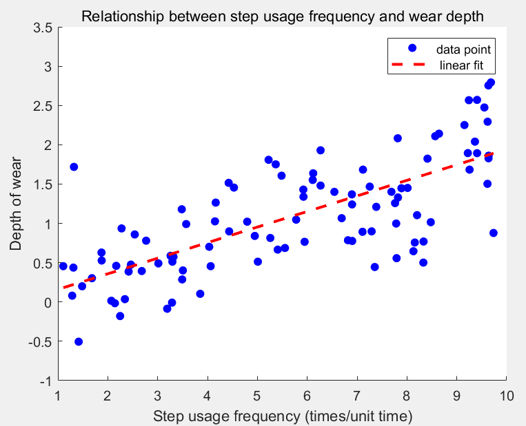
From the image, we can roughly observe that the influence weight of f(x₀,y₀)=6.25 on the wear depth is relatively large. In fact, after the error reduction calculation, the influence weight of f(x₀,y₀)=6.05 on the wear depth will be even greater. Therefore, the above calculation results can be verified.

3.1.2. Whether wear is consistent with available information

We have the actual wear data of 5 groups of stair steps and the predicted wear data obtained through the step wear model based on the existing information. At the same time, the threshold T = 1.5 is set to determine whether they are consistent. The data is shown in the following table 1:

For each set of data, we calculate the absolute value $$ |w_i-\widehat{w_i}|$$ of the difference between the actual wear value and the predicted wear value, and then determine x_ibased on the comparison result of this value with the threshold (x_i is a 0-1 variable, indicating whether the wear condition of the i-th set of data is consistent with the existing information). Due to the large amount of data, we select one set of data for demonstration, and its calculation process is as follows:

Calculate the absolute value of the difference.:  $$ |w_i-\widehat{w_i}|$$ =|8.2-7.5|= 0.7

Compare with the threshold value: since 0.7≤1.5,then $$ x_1$$ =1.

The calculation results show that the wear conditions of steps 1, 3, and 4 are consistent with the existing information (x₁ = x₃ = x₄ = 1), while those of steps 2 and 5 are inconsistent with the existing information (x₂ = x₅ = 0). To further verify, we calculate the mean square error for the above five sets of data and conduct a residual analysis. The calculation process is as follows:

Calculate the residual for each sample. $$ e_i=w_i-{\hat{w}}_i$$ ,

Calculate the square of each residual.  $$ e_i^2$$ ,

Calculate the mean square error MSE: $$ MSE=\frac{1}{5}\times 8.23=1.646$$ .

From the perspective of measurement accuracy for stair wear, if the measuring tool has a precision of one decimal place , an MSE of 1.646 is relatively large. This is because the square root of MSE, approximately 1.28, exceeds the tool's precision range. This suggests that the model's prediction accuracy needs improvement and may not be acceptable.

If the measurement accuracy itself is relatively low, for instance, the measurement error is ±1 or even larger, then MSE = 1.646 might be acceptable, indicating that the error of the model's prediction is at a relatively comparable level to the error of the measurement itself, and the model has a certain degree of rationality.

3.1.3. Step age estimation

We have collected research results related to historical verification and radiocarbon dating, and have obtained the following comparative data, the results are shown in Table 2.

Reliability analysis was conducted by comparing two sets of data: historical verification and radiocarbon dating. The natural wear rate could be obtained through material properties (wood, stone) and wear characteristics (friction coefficient, durability). The data was linearly fitted using MATLAB, and the following results were obtained. The results are shown in Figure 3.

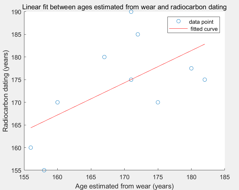
The fitting curve shows the trend of the linear relationship between the estimated age based on wear and the radiocarbon dating age. The data points are not closely clustered around the fitting curve, indicating that there is not a strong linear correlation between the two, that is, the estimated age based on material wear and the radiocarbon dating age are not completely consistent to a certain extent.

3.1.4. Repairs and innovations

We have collected research results related to X-ray analysis and infrared imaging, and quantified their data. The calculation process for X-ray analysis is as follows: For each X-ray image of the staircase samples, it is divided into n×n small regions (here n=100), and the average gray value  $$ G_{ij}$$  of each small region is calculated, where i and j respectively represent the row and column indices of the small region in the image.

Calculate the average gray level of the entire image: $$ G_{avg}=\frac{1}{n^2}{\sum }_{i=1}^n{\sum }_{j=1}^n{G}_{ij}$$ 

Calculate the standard deviation of the grayscale values: $$ \sigma =\sqrt{\frac{1}{n^2}{\sum }_{i=1}^n{\sum }_{j=1}^n(G_{ij}-G_{avg}{)}^2}$$ 

The standard deviation σ is used to measure the dispersion of the gray values, that is, the uniformity of wear. The smaller the σ value, the more uniform the wear is. The infrared imaging calculation process is as follows: Extract the temperature data of each stair sample surface from the infrared thermal imaging image. Similarly, divide the image into m×m small areas (here m=50), and record the temperature value $$ T_{ij}$$ of each small area.

Calculate the average temperature of the entire image: $$ Tavg=\frac{1}{m^2}{\sum }_{i=1}^m{\sum }_{j=1}^m{T}_{ij}$$ 

Calculate the standard deviation of the temperature: $$ \delta =\sqrt{\frac{1}{m^2}{\sum }_{i=1}^m{\sum }_{j=1}^m(T_{ij}-T_{avg}{)}^2}$$ 

The smaller the  $$ \delta $$ value is, the more uniform the temperature distribution is, which means the surface wear is more uniform.

Combining the results from both analysis methods, we find that the new staircase has smaller standard deviations in X-ray gray values and infrared temperature readings compared to the old staircase, which shows larger deviations in both metrics.In conclusion, the new staircase appears intact with no significant signs of repair or renovation, aside from minor surface treatments. In contrast, the old staircase exhibits various signs of repair and renovation, including material replacement, structural reinforcement, and surface restoration.

3.1.5. Identify the source of materials

Let's assume that there are m₁ types of elements in elemental analysis, m₂ isotopes in isotope analysis, m₃ tree-ring data points in tree-ring analysis, and m₄ texture feature parameters in texture analysis. Then, the calculation formula for the loss index I is:

Where z_1j is the jth influencing factor data of the standardized staircase material sample, and z_2j is the jth influencing factor data of the standardized suspected original source material sample.

When the loss index I is small (e.g., I < 0.1), it indicates that the chemical composition and texture of the staircase material closely match those of the suspected original source, with consistent wear. When I is large (e.g., I > 0.5), significant differences exist between the two. For intermediate values (0.1 ≤ I ≤ 0.5), the situation is more complex and uncertain.We demonstrate this using data from a stone staircase sample and a suspected original quarry stone sample. The results are shown in Table 3.

After calculation, the loss index I = 0.2 can be obtained, which indicates that there is a certain difference between the two, but there is still a possibility that the stone of the staircase comes from this quarry.

3.2.  The impact of changes in pedestrian flow

3.2.1. People flow preference direction

To investigate whether people using stairs tend to favor a specific walking direction, we incorporated it into the human flow model n(x, y, t). For simplicity, we assume that the human flow is only related to the position x of the stairs (assuming the stairs are one-dimensional, representing the position from one end to the other) and time t, and the directional relationship v(x, t) is related to n(x, t).

We define the preference direction coefficient P to measure people's walking direction preference on the stairs. Suppose that within time t, the number of people moving from one end of the stairs (set as the x=0 end) to the other end (set as the x=L end) is N_forward (t), and the number of people moving in the opposite direction is N_forward (t), then the preference direction coefficient P is:

To calculate N_forward (t) and N_backward (t) , we integrate the human flow model n(x,t) in the corresponding direction. Assuming that the distribution of human flow on the staircase is continuous, and the movement direction is positive when it is the same as the positive direction of the x-axis.

Here,  $$ H\left(u\right)$$  is the Heaviside function, defined as:

If u $$ \ge $$ 0, $$ H\left(u\right)$$  =1;else  $$ H\left(u\right)$$  =0

Suppose the human flow model is $$ n(x,t)=10+2\mathit{sin}(\frac{\pi x}{L}\left)\mathit{sin}(\frac{\pi t}{T}\right)$$  (where T is the time period, assume T = 1 unit of time, and L is the length of the staircase, assume L = 10 units of length), and the directional relationship is  $$ v(x,t)=0.5+0.3\mathit{cos}(\frac{\pi x}{L}\left)\mathit{cos}(\frac{\pi t}{T}\right)$$ . First, calculate N_forward (t):

For the calculation similar to N_backward (t). Then calculate P(t).

For instance, at t = 0.5, calculate through numerical integration (such as using Simpson's rule):

where h =  $$ \frac{L}{H}$$ , N is the number of divisions of the integral interval (assuming N = 100),  $$ x_i=i\cdot h$$ 

$$ f\left(x\right)=10+2\mathit{sin}(\frac{\pi x}{10}\left)\mathit{sin}(\frac{\pi \times 0.5}{1}\right)$$ .

Calculate N_backward (t) in the same way and finally obtain P(0.5).

The preference direction coefficient P represents the degree to which people favor a specific direction when walking. When P = 0.5, it indicates no significant directional preference in the studied scenario based on the pedestrian flow model. For example, in stairway scenarios, the flow of people going up and down is roughly equal, or the likelihood of walking left or right is the same. Both unidirectional and bidirectional movements are possible at different times and positions, with no direction being significantly favored. To visualize this variation, we used MATLAB to create a heatmap, as shown in the following figure 4:

From the above image, we can clearly verify the uncertainty of the preference direction. To further test, we conducted a Spearman analysis on the referenced parameter data using SPSS, and the results are as shown in the following figure 5:

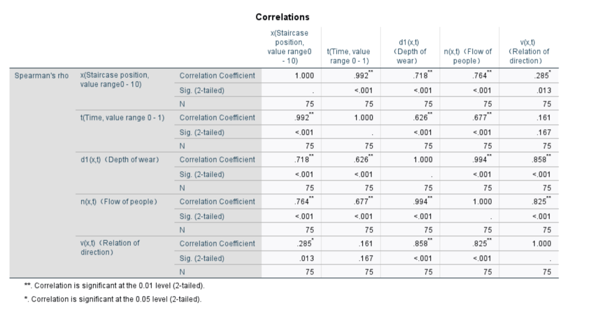
From the analysis of the data in the graph, it can be seen that the correlation coefficients between different factors vary significantly, further verifying the randomness presented in the preference direction.

3.2.2. Predict the number of people using the steps

By integrating the research achievements of LWR traffic flow and queuing theory, we can obtain the following set data, The results are shown in Table 4.

Suppose the function f(A_in,A_out)=0.8 related to the entrance and exit factors (derived through a comprehensive assessment of the size, quantity, and traffic capacity of the entrances and exits, etc.) is based on the human flow model :

$$ n(x,y)=\frac{w\cdot v\cdot \rho }{1+{{{\frac{l_q}{l_{max}}}^{-\frac{t_q}{t_{avg}}}}_{in}}_{out}}$$ .

We compute that  $$ 1-e^{-\frac{t_q}{t_{avg}}}=1-e^{-\frac{10}{20}}=1-e^{-0.5}\approx 1-0.6065=0.3935$$ . Then,we have  $$ w\cdot v\cdot \rho =2\times 0.5\times 2=2$$ . Substitute the above results into the formula of the pedestrian flow model. Suppose the observation time is T = 10 seconds, then the number of people using the stairs simultaneously during this period is approximately:

 $n=n(x,y)\times T=0.5277\times 10\approx 5\text{人}$ .

This means that approximately 0.5277 people pass through the staircase every second. Over a 10-second observation period, about 5 people use the staircase simultaneously. Given this result, it is unlikely that people are ascending in pairs (which would be in multiples of 2), and more likely that they are going up one after another. However, this is a speculation based on the current model and data; actual conditions may vary due to various factors.

3.2.3. Number of users per day

We obtained user data at different times of the day from surveillance cameras[3], access control systems, and pressure sensors. Suppose there are m data points: (t₁, n₁), (t₂, n₂), ..., (t_m, n_m). We use Mean Squared Error (MSE) to measure the difference between predicted values and actual data. For each time point t, if the model's predicted value is:

$$ \hat{n}\left(t_i\right)=A\mathit{sin}(w{t}_i+\varphi )+B$$ ,

then the Mean Squared Error is:

Then, the PSO (Particle Swarm Optimization) was carried out. The maximum number of iterations was set, and after optimization, the following results were obtained. The results are shown in Table 5.

From the result data, we can determine the peak and trough times for stair usage in a day, such as 8 a.m. (peak) and 10 p.m. (trough). The sine wave's fluctuation amplitude shows significant variation in the number of people at different times, indicating periods with large crowds in short intervals. Additionally, the data distribution reveals that usage is relatively low from midnight to morning, showing a prolonged period of low activity.

In addition, to make the data results more specific, we used MATLAB to perform a linear fit on the trend of the number of people using the stairs in a day, the results are shown in Figure 6.

This image demonstrates how the PSO (Particle Swarm Optimization) algorithm[5] is used to optimize the parameters of a sine wave periodic model to fit the actual data of the number of users. Eventually, the actual data and the fitted curve are plotted, visually presenting the trend of the number of people using the stairs throughout the day.

4.  Conclusion

The comprehensive analysis of the wear and tear of stairs, the flow of people and related factors is a very complex issue. Up to now, there are no accurate research results and comprehensive and detailed literature records on this issue. To give a satisfactory explanation of its inherent laws, more time and effort may be needed. We hope that the stair wear model, the flow of people model and the PSO particle swarm optimization model we have constructed can provide some help for the practical applications such as the design, maintenance and personnel flow management of stairs, and make some contributions to the research of ancient buildings. At the same time, we also hope that readers can give us some suggestions for improving the model.

References

[1]. Yue Jie. A Preliminary Study on the Expressiveness of the Staircase in the Michelangelo Laurenziana Library [J]. China Water Transport (Lower Half), 2009, 9 (06): 249-250.
[2]. Zhang Zhang. The Design of Shopping Mall Circulation Lines [M]. China Architecture & Building Press, 2017.
[3]. Yang Lizhong. The Movement Laws of People in Buildings and Evacuation Dynamics [M]. Science Press, 2012.
[4]. Kennedy J, Eberhart R C. Particle swarm optimization [C]//Proceedings of ICNN'95 - International Conference on Neural Networks. IEEE, 1995, 4 (1942 - 1948): 1942 - 1948.
[5]. Li X, Yao X. Evolutionary particle swarm optimizer with neighborhood - based topology [J]. IEEE Transactions on Evolutionary Computation, 2004, 8 (3): 204 - 212.
Cite this article
Li,D.;Wen,H.;Xu,J.;Li,C. (2025). Research on Stair Wear of Ancient Building. Applied and Computational Engineering,171,1-15.
Data availability
The datasets used and/or analyzed during the current study will be available from the authors upon reasonable request.
Disclaimer/Publisher's Note
The statements, opinions and data contained in all publications are solely those of the individual author(s) and contributor(s) and not of EWA Publishing and/or the editor(s). EWA Publishing and/or the editor(s) disclaim responsibility for any injury to people or property resulting from any ideas, methods, instructions or products referred to in the content.
About volume
Volume title: Proceedings of the 3rd International Conference on Functional Materials and Civil Engineering
© 2024 by the author(s). Licensee EWA Publishing, Oxford, UK. This article is an open access article distributed under the terms and
conditions of the Creative Commons Attribution (CC BY) license. Authors who
publish this series agree to the following terms:
1. Authors retain copyright and grant the series right of first publication with the work simultaneously licensed under a Creative Commons
Attribution License that allows others to share the work with an acknowledgment of the work's authorship and initial publication in this
series.
2. Authors are able to enter into separate, additional contractual arrangements for the non-exclusive distribution of the series's published
version of the work (e.g., post it to an institutional repository or publish it in a book), with an acknowledgment of its initial
publication in this series.
3. Authors are permitted and encouraged to post their work online (e.g., in institutional repositories or on their website) prior to and
during the submission process, as it can lead to productive exchanges, as well as earlier and greater citation of published work (See
Open access policy for details).