1. Introduction
The importance of early intervention and tailored teaching approaches is crucial for students with special needs. Elementary mathematics is a foundational skill that significantly influences academic achievement and long-term educational outcomes [1]. Research shows that early math proficiency predicts future success in STEM fields and socioeconomic status [2]. Despite approximately 7.5 million U.S. students aged 3-21 receiving special education services under IDEA during the 2022-23 school year—representing 15% of total public school enrollment—students with disabilities often face unique cognitive and instructional challenges that hinder their mathematical development, raising questions about the effectiveness of special education programs in addressing these issues [3, 4].
These challenges underscore the need for evidence-based interventions that are flexible and systematically applied. Special education techniques such as explicit instruction, hands-on learning tools, and assistive technology have shown promise in enhancing mathematical understanding for students with disabilities [5]. However, it should also be considered that students assigned to special education are usually taught mathematics that is different from that of regular education students [6]. This could correspond to Lekhal’s research in Norway finding that special education had little effect on improving standard math exam scores [7]. Ethical constraints preclude the use of Randomized Controlled Trials (RCTs) to assess the impact of special education services, necessitating reliance on observational study designs for empirical investigation. The observed differences in the aforementioned studies regarding the effects of special education on mathematical performance highlight a fundamental challenge in observational research—the difficulty in disentangling true intervention effects from spurious associations [8]. Causal inference allows researchers to move beyond simple statistical associations by accounting for confounding variables and constructing valid comparison groups [9, 10]. In education policy evaluation, such methods are essential for assessing the effectiveness of interventions [11]. At present, there are relatively few explorations based on causal inference to verify the effectiveness of special education in mathematics performance. Furthermore, socioeconomic status and educational background are well-established predictors of math achievement [12]. However, whether these factors differentially affect distinct subgroups within the special education population remains unexplored.
To rigorously examine the causal impact of special education on mathematics performance and investigate potential effect heterogeneity across socio-economic and educational background subgroups, this study employs longitudinal data from the Early Childhood Longitudinal Study Kindergarten 2010-11 cohort (ECLS-K:2011). Causal inference based on treatment effect will be introduced to verify the causality of special education on elementary mathematics outcomes. After data processing, the fundamental pipeline follows a "fit model + compute treatment effect" approach to achieve robust causal inference [13-15]. Traditional machine learning models with statistical interpretability such as Ordinary Least Squares method (OLS), Weighted Least Squares Regression, Bayesian Additive Regression Trees (BART), and Causal Forest will be employed.
The article is structured in the following manner: in Section 2, we first introduce the framework of causal inference. Hence, we introduce the combination of causal inference and traditional machine learning models by literature review. In Section 3, we employ an appropriate baseline model to verify the significance level of causal relationship under strong assumptions. Then Propensity Score Matching (PSM) techniques will be applied to eliminate selection bias [16]. Next, Bayesian-based models will be assessed to check the consistency of Frequentist and Bayesian Statistics [17]. After the identification of causality, Section 4 details further analysis of heterogeneous based on sub-population focusing on socioeconomic status and educational background. In Section 5, we present and analyze the causal effect estimates, evaluating their statistical significance through p-values and confidence intervals. In Section 6, we draw our conclusions.
2. Literature review
2.1. Causal frameworks
The primary objective of causal inference is to estimate the causal effects of treatments on outcomes, moving beyond mere correlation analysis. Modern causal inference is built upon two foundational frameworks: Rubin's Potential Outcomes Model and Pearl's Causal Diagrams [18, 19]. As a cornerstone of this field, the Potential Outcomes Framework establishes three key assumptions: (1) Stable Unit Treatment Value Assumption (SUTVA), which states that an individual's outcome remains unaffected by the treatment status of other individuals; (2) Ignorability, meaning that treatment assignment T becomes independent of potential outcomes when conditioned on covariates X; and (3) Overlap, ensuring that every individual has a non-zero probability of receiving either treatment or control [18]. Under these assumptions, causal effects can be formally quantified. The Average Treatment Effect (ATE) measures the expected outcome difference between treated and untreated groups across the entire population. Mathematically, let
The Conditional Average Treatment Effect (CATE), on the other hand, estimates treatment effects within subpopulations defined by covariates X, expressed as:
The CATE allows for heterogeneous treatment effect analysis, revealing how causal effects vary across different sub-segments of the population.
To address potential imbalances and selection bias between treatment and control groups, Rosenbaum and Rubin introduced the Propensity Score Matching (PSM), defined as
representing the probability of receiving treatment given observed covariates Xi [20]. By matching individuals with similar propensity scores across groups, researchers can approximate the conditions of a randomized experiment, thereby reducing confounding. Empirical studies have demonstrated that this approach yields estimates comparable to those from Randomized Controlled Trials (RCTs) in observational research [21-23].
2.2. Causal inference and machine learning
Recent years have witnessed a growing interest in integrating causal inference methodologies with traditional machine learning (ML) techniques for observational studies. This interdisciplinary approach has emerged as a powerful solution for addressing fundamental challenges in causal identification and estimation.
The methodological evolution in this field can be traced through several key developments. Rosenbaum and Rubin pioneered the use of Propensity Score Matching (PSM) through logistic regression, establishing a robust framework for addressing selection bias in observational data [20]. Building on this foundation, Athey and Imbens introduced causal trees, adapting decision tree algorithms for causal inference tasks [24]. This innovation was further advanced by Wager and Athey through the development of causal random forests, which implied random forests learning techniques into causal inference to determine heterogeneous effects [25]. Additionally, Hill et al. demonstrated the robustness of Bayesian Additive Regression Trees (BART) in estimating causal effects of medical coverage on health outcomes, highlighting the potential of Bayesian based model for causal inference.
Traditional ML models - including linear regression, logistic regression, and decision trees - offer distinct advantages for causal analysis due to their statistical interpretability [26, 27]. These methods provide essential inferential tools such as significance testing (p-values), confidence interval estimation, and hypothesis testing capabilities. Such features enable researchers to rigorously assess the robustness of estimated causal relationships, explaining their widespread adoption across social science research [28, 29].
3. Data description and preprocessing
3.1. Data description
The analysis uses the Early Childhood Longitudinal Study Kindergarten 2010-11 cohort (ECLS-K:2011) dataset, collected by the National Center for Education Statistics (U.S. Department of Education). After standard preprocessing (including the removal of cases with missing key variables and outliers), our analytical dataset includes 7,362 students, in which 429 received special education services by fifth grade (treatment group) and 6,933 did not (control group). The binary treatment indicator, F5SPECS, equals 1 if a student received any special education and 0 otherwise. Our outcome, C6R4MSCL, is the continuous fifth‑grade math assessment score, which ranges from 50.9 to 170.7. We will use a set of 34 covariates to adjust for confounding. These variables include six domains: Demographic, Academic, School composition, Family context, Health, and Parent rating of child. These covariates enable us to control various factors that may influence the likelihood of receiving special education services and math achievement.
3.2. Data preprocessing
Before causal inference analysis, we carried out three preprocessing steps to clean the ECLS‑K:2011 dataset, select the most relevant covariates, and reduce their dimensionality in a supervised manner. The entire process was implemented in R (version 4.3.1).
3.2.1. Variable selection via LASSO
Since our dataset involves 34 pre‑treatment covariates, to prevent overfitting and focus on the most outcome-predictive features, we used Least Absolute Shrinkage and Selection Operator (LASSO) Regression to select the covariates that best predict the outcome [30, 31]. All covariates were first standardized to mean zero and unit variance. We then fitted a penalized linear model by solving,
Where
3.2.2. Supervised dimension reduction with PLS
To condense LASSO‑selected predictors into a small number of orthogonal, outcome‑relevant features, we further utilize Partial Least Squares (PLS) regression [33]. PLS can construct each latent component
3.2.3. Diagnostic visualizations
To demonstrate the effect of dimension reduction, we compare before‑and‑after correlation structures and examine the PLS components themselves. We compared the raw 34‑variable correlation matrix and the reduced correlation matrix (outcome, treatment, and PLS components) in Figure 1, illustrating that the five components are largely orthogonal and remove spurious correlations. We also performed a quick PCA on this correlation matrix to confirm that each PLS component aligns with distinct, high‑variance directions in Figure 2, validating that our supervised reduction successfully captured the dominant covariate patterns without redundancy.
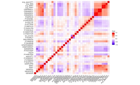
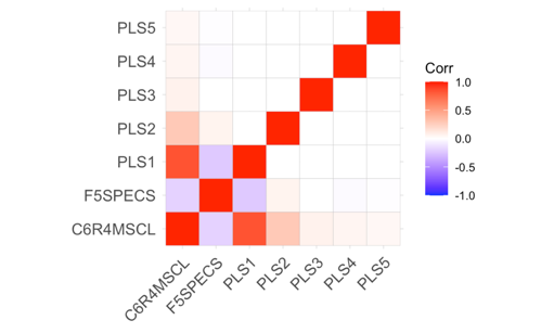
Figure 1. Correlation heatmap
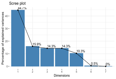
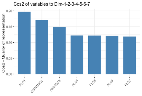
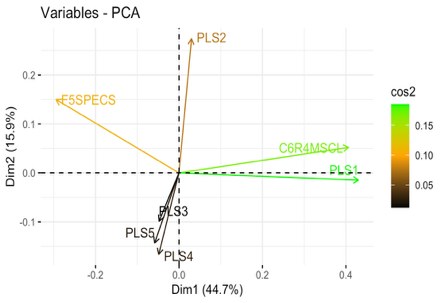
Figure 2. Validation plots
Together, these preprocessing steps ensure that our causal inference models operate on a compact, orthogonal set of covariates that are both predictive of the outcome and robust against confounding, thereby laying a solid foundation for unbiased ATE and CATE estimation.
4. Methods
With a set of five orthogonal covariates, we proceeded to estimate both Average Treatment Effects (ATE) and Conditional Average Treatment Effects (CATE). We have included the following methods: (1) Linear regression with the Ordinary Least Squares method (OLS), (2) Propensity Score Matching (PSM, including logistic regression, k-nearest neighbor algorithm), (3) Bayesian Additive Regression Trees (BART) and (4) Causal Forest.
4.1. Ordinary least squares regression
We first specify a baseline linear regression model to estimate the average treatment effect (ATE). The model is formulated as:
where
4.2. Propensity score matching
To approximate a randomized experiment and mitigate selection bias, we implement Propensity Score Matching (PSM) [20, 36]. The propensity score for each student is defined as the probability of receiving special education services conditional on their pre‑treatment covariates:
Here
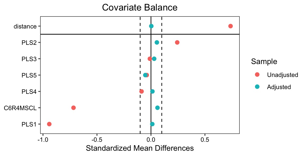
Using these estimated propensities, we perform one‑to‑one nearest‑neighbor matching without replacement, imposing a caliper of 0.2 standard deviations of the logit of the propensity score to avoid poor matches [20, 37]. After matching, we verify covariate balance by comparing standardized mean differences for each PLS component before and after matching, visualized via a love plot in Figure 3.
4.3. Bayesian additive regression trees
To provide a fully Bayesian complement to our nonparametric forests, we implement Bayesian Additive Regression Trees (BART) [38]. BART represents the outcome surface as a sum of regression trees,
where each tree
We fit two separate BART models in an “augmented” framework for causal inference, one is “Control Model”
4.4. Causal forest
The Causal Forest model is an extension of the Random Forest model, designed to predict the relationship between outcome variables and covariates by constructing multiple decision trees [39]. During the training process, each tree randomly selects features and samples, enabling the model to effectively capture complex nonlinear relationships and interactions within the data.
In addition to addressing nonlinearity, this model is particularly well-suited for estimating the variation in treatment effects across different individuals or subgroups. Causal Forest model provides a more nuanced understanding of the specific distribution of treatment effects by estimating Individual Treatment Effects (ITE). Let us denote the outcome variable as Y, the treatment variable as D, and the covariate variables as W. We can represent the model prediction for each individual as
The distributional information derived from ITE estimations can facilitate a range of valuable statistical inferences. Furthermore, the ATE can be estimated by taking the mean of the ITE estimates.
5. Results and analysis
5.1. Descriptive statistics
|
Math Score |
PLS1 |
PLS2 |
PLS3 |
PLS4 |
PLS5 |
|
|
Control (n=6933) |
128.19 ( |
2.36 ( |
-0.21 ( |
0.01 ( |
0.06 ( |
0.01 ( |
|
Treated (n=429) |
108.97 ( |
-38.10 ( |
3.44 ( |
-0.17 ( |
-1.02 ( |
-0.17 ( |
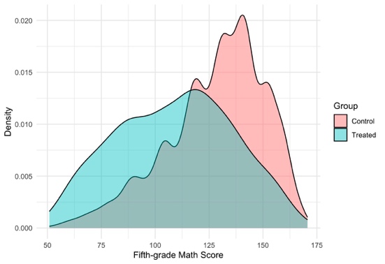
Table 1 and Figure 4 jointly highlight significant pre-treatment imbalances between treated and control groups, with a nearly 19-point gap in average math scores and substantial differences in PLS1, which captures academic and health characteristics, along with smaller but consistent disparities in PLS2–PLS5; the density plot further illustrates that treated students are concentrated in lower score ranges, reinforcing the necessity of applying matching or other adjustment techniques to ensure unbiased causal estimates.
5.2. Average treatment effects (ATE)
|
Math Score |
PLS1 |
PLS2 |
PLS3 |
PLS4 |
PLS5 |
|
|
Control (n=6933) |
128.19 ( |
2.36 ( |
-0.21 ( |
0.01 ( |
0.06 ( |
0.01 ( |
|
Treated (n=429) |
108.97 ( |
-38.10 ( |
3.44 ( |
-0.17 ( |
-1.02 ( |
-0.17 ( |
The Ordinary Least Squares method (OLS) estimate for the treatment indicator (F5SPECS) is -1.60 (SE = 0.57, p=0.0048), indicating that, after adjusting for the five PLS components, students who received special education services score on average 1.6 points lower in fifth‑grade math than their non‑treated peers. The model explains about 77.5% of the variance in math scores, and the orthogonality of the PLS covariates keeps multicollinearity at bay.
However, this OLS result remains an associational estimate. It relies on the strong assumption of no unmeasured confounding: any omitted variable correlated with both treatment assignment and the outcome could bias
5.2.1. Ordinary Least Squares (OLS)
|
Estimate |
Std. Error |
t-value |
p-value |
|
|
Intercept |
127.165 |
0.134 |
952.45 |
<0.001 |
|
Treatment |
-1.605 |
0.569 |
-2.82 |
0.0048 |
|
PLS1 |
0.473 |
0.003 |
144.81 |
<0.001 |
|
PLS2 |
0.463 |
0.009 |
51.06 |
<0.001 |
|
PLS3 |
0.098 |
0.008 |
12.46 |
<0.001 |
|
PLS4 |
0.098 |
0.011 |
9.12 |
<0.001 |
|
PLS5 |
0.209 |
0.028 |
7.47 |
<0.001 |
|
R2 |
0.775 |
|||
|
Adj. R2 |
0.774 |
|||
|
Observations |
7,362 |
|||
The OLS estimate for the treatment indicator (F5SPECS) is -1.60 (SE = 0.57, p=0.0048), indicating that, after adjusting for the five PLS components, students who received special education services score on average 1.6 points lower in fifth‑grade math than their non‑treated peers. The model explains about 77.5% of the variance in math scores, and the orthogonality of the PLS covariates keeps multicollinearity at bay.
However, this OLS result remains an associational estimate. It relies on the strong assumption of no unmeasured confounding: any omitted variable correlated with both treatment assignment and the outcome could bias
5.2.2. Propensity score matching
|
Estimate |
Std. Error |
t-value |
p-value |
|
|
Survey-weighted regression (svyglm) |
-0.687 |
1.822 |
-0.377 |
0.706 |
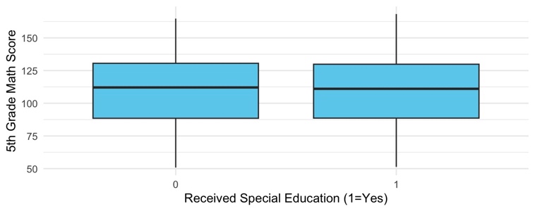
Table 4 contrasts sharply with the OLS estimate of ATE = –1.60 (p = 0.0048): using PSM, the estimated treatment effect becomes -0.6867 but remains statistically insignificant (p = 0.707). To confirm adequate common support, Figure 8 displays box plots of fifth‑grade math scores in the matched sample. The considerable overlap in score distributions between treated and control students indicates that matching on the PLS covariates was successful. This reversal in sign—from a significant negative association in the uncontrolled OLS to a small, positive but imprecise estimate after matching—underscores how baseline imbalances drove the negative OLS result and highlight the importance of covariate balance for valid causal inference.
5.2.3. Bayesian additive regression trees
|
Posterior Mean |
Posterior Median |
95% Credible Interval |
|
|
Full Data Set |
-0.2525 |
-0.2689 |
[1.7619, 1.6477] |
|
Matched Data Set |
-1.1484 |
-1.1346 |
[-2.5711, 0.5010] |
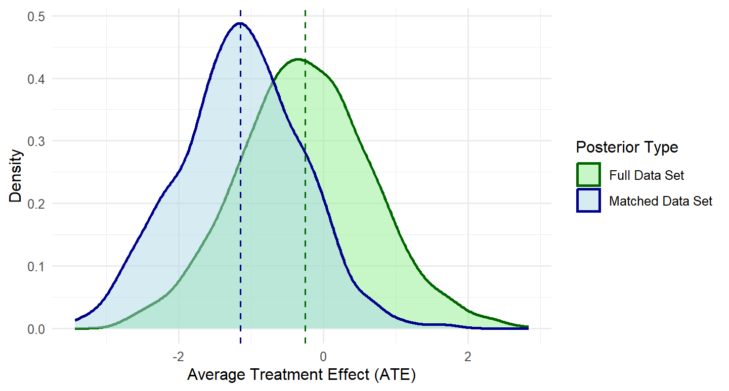
The BART model was applied to both the original full dataset and the PSM dataset to estimate treatment effects. Cross-validation results suggested that 50 trees provided optimal model performance. As presented in Table 5, comparative analysis of the estimation outcomes between these two datasets demonstrates that PSM effectively reduces selection bias in the observational study. Notably, the posterior distributions reveal consistently negative treatment effects in the matched-data-based model, whereas the full-dataset-based model yields only marginally negative estimates. This differential pattern shades light on the importance of accounting for selection bias through matching procedures.
5.3. Heterogeneity analysis by CATE
Although our ATE estimates were small and imprecise, special education services may nonetheless benefit certain subpopulations more than others. We therefore use Causal Forest to estimate Conditional Average Treatment Effects (CATE) as a function of two groups of key moderators: 1. Early academic ability (kindergarten math IRT score, MIRT) and school sector (public vs. non-public, S2KPUPRI), 2. Family socioeconomic status.
5.3.1. Heterogeneity by educational background
|
Estimate |
Std. Error |
t-value |
p-value |
|
|
Intercept |
-1.81933 |
0.04830 |
-37.665 |
<0.001 |
|
Kindergarten Math Score |
0.03501 |
0.00113 |
30.981 |
<0.001 |
|
Public School |
0.10859 |
0.02761 |
3.933 |
<0.001 |
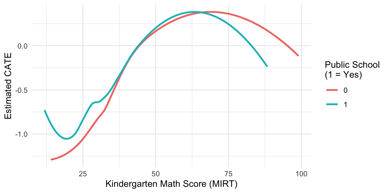
The moderator regression yields highly significant coefficients (both p<0.001). This indicates that each additional point on the kindergarten math IRT score (MIRT) raises the estimated treatment effect by about 0.035 points, while attending a public school adds roughly 0.11 points to the CATE. Figure 10 plots of these fitted CATE curve against MIRT for public versus non-public students. In both settings, treatment effects start negative at low ability, peak around mid-range scores (MIRT≈50–70), and decline again for the highest-ability learners. Notably, public-school students suffer fewer negative effects at the lowest ability levels, whereas non-public students maintain higher effects at the top end.
5.3.2. Heterogeneity by socioeconomic background
|
No |
Yes |
|
|
If step parent |
-0.5425 |
-0.4755 |
|
If single parent |
-0.5857 |
-0.7938 |
|
If received food stamp |
-0.4937 |
-0.8487 |

The dataset includes family-related socioeconomic indicators that may lead to heterogeneous treatment effects. Of particular interest are three key variables: single-parent status, stepparent family structure, and food stamp receipt. These factors are highly correlated with family background and could well reflect the socioeconomic situation. As shown in Table 6, the causal forest model estimates distinct CATEs for these family structure indicators. The results demonstrate weak variations in treatment effects based on family backgrounds. Since the characteristics of Causal Forest model, distribution of ITE under family backgrounds condition are plotted for CATE estimation. From the density shape, both scale and location reveal difference within corresponding subgroups. Confident intervals based on T-test shown in Table 9 further suggest the existence of heterogeneity. Specifically, children from non-single parent families and families that do not receive food stamps have a significant advantage in ITE, while children from stepparent families have a significant difference in ITE. However, the presence of both positive and negative values in the confidence interval diminishes the advantage of IDE in stepparent subgroup. The analysis of these three subcategories indicates that under more favorable socioeconomic conditions, the treatment effect of special education will exhibit stronger effects.
|
If step parent |
[0.240, 0.359] |
|
If single parent |
[-0.203, 0.005] |
|
If received food stamp |
[0.251, 0.390] |
6. Discussion
6.1. Key findings
Our analysis began with an innovative data-preprocessing and dimension-reduction strategy that combined LASSO variable selection and supervised PLS extraction. We first used LASSO to winnow the original 34 covariates down to those most predictive of fifth-grade math performance, then applied PLS to compress these into five orthogonal components, thereby eliminating multicollinearity and furnishing a compact, high-information basis for our causal models (see Figures 1-5).
Applying this framework, OLS results suggested a significant negative association (-1.60 points, p=0.0048), but this was likely confounded by baseline imbalances. After adjusting for selection bias via Propensity Score Matching (PSM), the effect changed to -0.69, becoming statistically insignificant (p=0.707), showing the role of covariate balance in causal inference. Bayesian Additive Regression Trees (BART) on matched data reinforced the weak negative effect, underscoring the need for nonparametric methods to handle potential nonlinearities. Furthermore, the discrepancy between the BART estimates on the full dataset and the OLS results further highlights the fundamental methodological divergence between frequentist and Bayesian methods.
CATE analysis via Causal Forest reveals heterogeneity in treatment effects based on students’ educational background and socioeconomic structure. Specifically, each additional point in kindergarten math ability (MIRT) increases the predicted effect of special education by about 0.0035, with the most positive impacts concentrated among students with mid-level readiness (MIRT = 50-70). Moreover, indicators of socioeconomic background (including single-parent status, stepparent households, and food stamp receipt) showed significant moderating influence. The differences in distribution shape of CATE and the results of T-test indicate that better socioeconomic conditions will have a positive impact on the treatment effect of special education.
6.2. Policy implications
These findings carry important implications for policy and practice. Rather than a one-size-fits-all model, special education resources should be strategically targeted. Mid-ability students should remain a core focus, while very low-ability students in non-public settings need enhanced wrap-around support to prevent declines. High-ability learners require advanced enrichment rather than standard remediation. Finally, public schools’ success in buffering negative effects for the most vulnerable suggests their collaborative support models could be adapted by private programs.
6.3. Limitations and future directions
Several limitations may affect our conclusions. We focus exclusively on a single math outcome at grade five, leaving longer-term and non-cognitive impacts unexplored. Future research should extend this framework by mapping heterogeneity across disability types, intervention intensities, and longitudinal trajectories, as well as investigating mediating mechanisms (like improvements in attention or self-regulation) and testing the generalizability of findings across different school systems and international contexts.
6.4. Conclusion
In summary, our study demonstrates that average treatment effects can conceal critical variation in who benefits from special education. By integrating LASSO-PLS preprocessing, Propensity Score Matching (PSM), Bayesian Additive Regression Trees (BART), and machine-learning-based causal forests, we uncover that academic readiness, school sector and family background, drive heterogeneity in outcomes. This precision-targeting framework can help educators and policymakers allocate precision special education resources more effectively, narrowing achievement gaps and promoting educational equity.
References
[1]. Duncan, G. J., Dowsett, C. J., Claessens, A., Magnuson, K., Huston, A. C., Klebanov, P., Pagani, L. S., Feinstein, L., Engel, Sexton, H., Duckworth, K., & Japel,
[2]. Claesens, A., & Engel, M. (2013). How important is where you start? Early mathematics knowledge and later school success. Teachers College Record, 115(6), 1–29.
[3]. Lindsay, G. (2007). Student researchers in the middle: using visual images to make sense of inclusive education. Journal of Research in Special Educational Needs, 7(3), 145-154.
[4]. National Center for Education Statistics. (2023). Students with disabilities receiving special education services. U.S. Department of Education. https: //nces.ed.gov/programs/coe/indicator/cgg
[5]. Bouck, E. C., Park, J., & Nickell, B. (2017). Concrete-representational-abstract (CRA) instruction for students with math disabilities. Remedial and Special Education, 38(6), 357–369. https: //doi.org/10.1177/0741932517721712
[6]. Ballin, A., Davidson, E., Caron, J., & Drago, M. (2022). Making Math Add up for Students Receiving Special Education. International Journal of Whole Schooling, 18(1), 1-28.
[7]. Lekhal, R. (2018). Does special education predict students’ math and language skills?. European journal of special needs education, 33(4), 525-540.
[8]. Morgan, S. L., & Winship, C. (2015). Counterfactuals and causal inference: Methods and principles for social research (2nd ed.). Cambridge University Press.
[9]. Imbens, G. W., & Rubin, D. B. (2015). "Causal Inference in Statistics, Social, and Biomedical Sciences." Cambridge University Press.
[10]. Holland, P. W. (1986). Statistics and causal inference. Journal of the American statistical Association, 81(396), 945-960
[11]. Schneider, B., Carnoy, M., Kilpatrick, J., Schmidt, W. H., & Shavelson, R. J. (2017). Methods for estimating causal effects in education. Educational Researcher, 46(4), 207-212. https: //doi.org/10.3102/0013189X17703985
[12]. Papanastasiou, C. (2002). Effects of background and school factors on the mathematics achievement. Educational research and evaluation, 8(1), 55-70.
[13]. Rubin, D. B. (1980). Randomization analysis of experimental data: The Fisher randomization test comment. Journal of the American statistical association, 75(371), 591-593.
[14]. Rubin, D. B. (2005). Causal inference using potential outcomes: Design, modeling, decisions. Journal of the American Statistical Association, 100(469), 322-331.
[15]. Pearl, J. (2018). Theoretical impediments to machine learning with seven sparks from the causal revolution. arXiv preprint arXiv: 1801.04016.
[16]. Rubin, D. B. (1977). Assignment to treatment group on the basis of a covariate. Journal of educational Statistics, 2(1), 1-26.
[17]. Rubin, D. B. (1978). Bayesian inference for causal effects: The role of randomization. The Annals of statistics, 34-58.
[18]. Rubin, D. B. (1974). "Estimating Causal Effects of Treatments in Randomized and Nonrandomized Studies." Journal of Educational Psychology, 66(5), 688-701.
[19]. Pearl, J. (2009). "Causality: Models, Reasoning, and Inference." 2nd Edition. Cambridge University Press. DOI: 10.1017/CBO9781139167161
[20]. Rosenbaum, P. R., & Rubin, D. B. (1983). The central role of the propensity score in observational studies for causal effects. Biometrika, 70(1), 41-55.
[21]. Dehejia, R. H., & Wahba, S. (2002). Propensity score matching methods for non-experimental causal studies. Review of Economics and Statistics, 84(1), 151-161.
[22]. Smith, J. A., & Todd, P. E. (2005). Does matching overcome LaLonde's critique of nonexperimental estimators? Journal of Econometrics, 125(1-2), 305-353.
[23]. Stuart, E. A., Huskamp, H. A., Duckworth, K., Simmons, J., Song, Z., Chernew, M. E., & Barry, C. L. (2014). Using propensity scores in difference-in-differences models to estimate the effects of a policy change. Health Services and Outcomes Research Methodology, 14(4), 166-182.
[24]. Athey, S., & Imbens, G. (2016). Recursive partitioning for heterogeneous causal effects. PNAS, 113(27), 7353-7360.
[25]. Wager, S., & Athey, S. (2018). Estimation and inference of heterogeneous treatment effects using random forests. Journal of the American Statistical Association, 113(523), 1228-1242.
[26]. Molnar, C. (2020). Interpretable Machine Learning. https: //christophm.github.io/interpretable-ml-book/
[27]. Ribeiro, M.T., Singh, S., & Guestrin, C. (2016). "Why Should I Trust You?" Explaining the Predictions of Any Classifier. KDD.
[28]. Angrist, J.D. & Pischke, J.S. (2008). Mostly Harmless Econometrics. Princeton UP.
[29]. Imbens, G.W. & Rubin, D.B. (2015). Causal Inference for Statistics, Social, and Biomedical Sciences. Cambridge UP.
[30]. Tibshirani, R. (1996). Regression shrinkage and selection via the lasso. Journal of the Royal Statistical Society Series B: Statistical Methodology, 58(1), 267-288.
[31]. Muthukrishnan, R., & Rohini, R. (2016, October). LASSO: A feature selection technique in predictive modeling for machine learning. In 2016 IEEE international conference on advances in computer applications (ICACA) (pp. 18-20). Ieee.
[32]. Stone, M. (1974). Cross‐validatory choice and assessment of statistical predictions. Journal of the royal statistical society: Series B (Methodological), 36(2), 111-133.
[33]. Geladi, P., & Kowalski, B. R. (1986). Partial least-squares regression: a tutorial. Analytica chimica acta, 185, 1-17.
[34]. Kettaneh, N., Berglund, A., & Wold, S. (2005). PCA and PLS with very large data sets. Computational Statistics & Data Analysis, 48(1), 69-85.
[35]. Seber, G. A., & Lee, A. J. (2003). Linear regression analysis. John Wiley & Sons.
[36]. Caliendo, M., & Kopeinig, S. (2008). Some practical guidance for the implementation of propensity score matching. Journal of economic surveys, 22(1), 31-72.
[37]. Ho, D., Imai, K., King, G., & Stuart, E. A. (2011). MatchIt: nonparametric preprocessing for parametric causal inference. Journal of statistical software, 42, 1-28.
[38]. Chipman, H. A., George, E. I., & McCulloch, R. E. (2010). BART: Bayesian additive regression trees.
[39]. Splawa-Neyman, J., Dabrowska, D. M., & Speed, T. P. (1990). On the application of probability theory to agricultural experiments. Essay on principles. Section 9. Statistical Science, 465-472.
Cite this article
Li,L.;Su,X. (2025). Causal Machine Learning for Special Education: Estimating Heterogeneous Effects on Elementary Math Achievement. Applied and Computational Engineering,164,246-261.
Data availability
The datasets used and/or analyzed during the current study will be available from the authors upon reasonable request.
Disclaimer/Publisher's Note
The statements, opinions and data contained in all publications are solely those of the individual author(s) and contributor(s) and not of EWA Publishing and/or the editor(s). EWA Publishing and/or the editor(s) disclaim responsibility for any injury to people or property resulting from any ideas, methods, instructions or products referred to in the content.
About volume
Volume title: Proceedings of CONF-CDS 2025 Symposium: Data Visualization Methods for Evaluation
© 2024 by the author(s). Licensee EWA Publishing, Oxford, UK. This article is an open access article distributed under the terms and
conditions of the Creative Commons Attribution (CC BY) license. Authors who
publish this series agree to the following terms:
1. Authors retain copyright and grant the series right of first publication with the work simultaneously licensed under a Creative Commons
Attribution License that allows others to share the work with an acknowledgment of the work's authorship and initial publication in this
series.
2. Authors are able to enter into separate, additional contractual arrangements for the non-exclusive distribution of the series's published
version of the work (e.g., post it to an institutional repository or publish it in a book), with an acknowledgment of its initial
publication in this series.
3. Authors are permitted and encouraged to post their work online (e.g., in institutional repositories or on their website) prior to and
during the submission process, as it can lead to productive exchanges, as well as earlier and greater citation of published work (See
Open access policy for details).
References
[1]. Duncan, G. J., Dowsett, C. J., Claessens, A., Magnuson, K., Huston, A. C., Klebanov, P., Pagani, L. S., Feinstein, L., Engel, Sexton, H., Duckworth, K., & Japel,
[2]. Claesens, A., & Engel, M. (2013). How important is where you start? Early mathematics knowledge and later school success. Teachers College Record, 115(6), 1–29.
[3]. Lindsay, G. (2007). Student researchers in the middle: using visual images to make sense of inclusive education. Journal of Research in Special Educational Needs, 7(3), 145-154.
[4]. National Center for Education Statistics. (2023). Students with disabilities receiving special education services. U.S. Department of Education. https: //nces.ed.gov/programs/coe/indicator/cgg
[5]. Bouck, E. C., Park, J., & Nickell, B. (2017). Concrete-representational-abstract (CRA) instruction for students with math disabilities. Remedial and Special Education, 38(6), 357–369. https: //doi.org/10.1177/0741932517721712
[6]. Ballin, A., Davidson, E., Caron, J., & Drago, M. (2022). Making Math Add up for Students Receiving Special Education. International Journal of Whole Schooling, 18(1), 1-28.
[7]. Lekhal, R. (2018). Does special education predict students’ math and language skills?. European journal of special needs education, 33(4), 525-540.
[8]. Morgan, S. L., & Winship, C. (2015). Counterfactuals and causal inference: Methods and principles for social research (2nd ed.). Cambridge University Press.
[9]. Imbens, G. W., & Rubin, D. B. (2015). "Causal Inference in Statistics, Social, and Biomedical Sciences." Cambridge University Press.
[10]. Holland, P. W. (1986). Statistics and causal inference. Journal of the American statistical Association, 81(396), 945-960
[11]. Schneider, B., Carnoy, M., Kilpatrick, J., Schmidt, W. H., & Shavelson, R. J. (2017). Methods for estimating causal effects in education. Educational Researcher, 46(4), 207-212. https: //doi.org/10.3102/0013189X17703985
[12]. Papanastasiou, C. (2002). Effects of background and school factors on the mathematics achievement. Educational research and evaluation, 8(1), 55-70.
[13]. Rubin, D. B. (1980). Randomization analysis of experimental data: The Fisher randomization test comment. Journal of the American statistical association, 75(371), 591-593.
[14]. Rubin, D. B. (2005). Causal inference using potential outcomes: Design, modeling, decisions. Journal of the American Statistical Association, 100(469), 322-331.
[15]. Pearl, J. (2018). Theoretical impediments to machine learning with seven sparks from the causal revolution. arXiv preprint arXiv: 1801.04016.
[16]. Rubin, D. B. (1977). Assignment to treatment group on the basis of a covariate. Journal of educational Statistics, 2(1), 1-26.
[17]. Rubin, D. B. (1978). Bayesian inference for causal effects: The role of randomization. The Annals of statistics, 34-58.
[18]. Rubin, D. B. (1974). "Estimating Causal Effects of Treatments in Randomized and Nonrandomized Studies." Journal of Educational Psychology, 66(5), 688-701.
[19]. Pearl, J. (2009). "Causality: Models, Reasoning, and Inference." 2nd Edition. Cambridge University Press. DOI: 10.1017/CBO9781139167161
[20]. Rosenbaum, P. R., & Rubin, D. B. (1983). The central role of the propensity score in observational studies for causal effects. Biometrika, 70(1), 41-55.
[21]. Dehejia, R. H., & Wahba, S. (2002). Propensity score matching methods for non-experimental causal studies. Review of Economics and Statistics, 84(1), 151-161.
[22]. Smith, J. A., & Todd, P. E. (2005). Does matching overcome LaLonde's critique of nonexperimental estimators? Journal of Econometrics, 125(1-2), 305-353.
[23]. Stuart, E. A., Huskamp, H. A., Duckworth, K., Simmons, J., Song, Z., Chernew, M. E., & Barry, C. L. (2014). Using propensity scores in difference-in-differences models to estimate the effects of a policy change. Health Services and Outcomes Research Methodology, 14(4), 166-182.
[24]. Athey, S., & Imbens, G. (2016). Recursive partitioning for heterogeneous causal effects. PNAS, 113(27), 7353-7360.
[25]. Wager, S., & Athey, S. (2018). Estimation and inference of heterogeneous treatment effects using random forests. Journal of the American Statistical Association, 113(523), 1228-1242.
[26]. Molnar, C. (2020). Interpretable Machine Learning. https: //christophm.github.io/interpretable-ml-book/
[27]. Ribeiro, M.T., Singh, S., & Guestrin, C. (2016). "Why Should I Trust You?" Explaining the Predictions of Any Classifier. KDD.
[28]. Angrist, J.D. & Pischke, J.S. (2008). Mostly Harmless Econometrics. Princeton UP.
[29]. Imbens, G.W. & Rubin, D.B. (2015). Causal Inference for Statistics, Social, and Biomedical Sciences. Cambridge UP.
[30]. Tibshirani, R. (1996). Regression shrinkage and selection via the lasso. Journal of the Royal Statistical Society Series B: Statistical Methodology, 58(1), 267-288.
[31]. Muthukrishnan, R., & Rohini, R. (2016, October). LASSO: A feature selection technique in predictive modeling for machine learning. In 2016 IEEE international conference on advances in computer applications (ICACA) (pp. 18-20). Ieee.
[32]. Stone, M. (1974). Cross‐validatory choice and assessment of statistical predictions. Journal of the royal statistical society: Series B (Methodological), 36(2), 111-133.
[33]. Geladi, P., & Kowalski, B. R. (1986). Partial least-squares regression: a tutorial. Analytica chimica acta, 185, 1-17.
[34]. Kettaneh, N., Berglund, A., & Wold, S. (2005). PCA and PLS with very large data sets. Computational Statistics & Data Analysis, 48(1), 69-85.
[35]. Seber, G. A., & Lee, A. J. (2003). Linear regression analysis. John Wiley & Sons.
[36]. Caliendo, M., & Kopeinig, S. (2008). Some practical guidance for the implementation of propensity score matching. Journal of economic surveys, 22(1), 31-72.
[37]. Ho, D., Imai, K., King, G., & Stuart, E. A. (2011). MatchIt: nonparametric preprocessing for parametric causal inference. Journal of statistical software, 42, 1-28.
[38]. Chipman, H. A., George, E. I., & McCulloch, R. E. (2010). BART: Bayesian additive regression trees.
[39]. Splawa-Neyman, J., Dabrowska, D. M., & Speed, T. P. (1990). On the application of probability theory to agricultural experiments. Essay on principles. Section 9. Statistical Science, 465-472.


