1. Introduction

In the past decade, Internet finance has developed rapidly, especially the customer’s financial products. The financial industry is facing richer data and faster transactions. Given the technology nowadays, targeting specific customers with customized financial products is possible [1]. Banks can use statistical information to develop products or carry out marketing activities suitable for their target customers. Customized financial product advertising can aim directly at customers and provide unique personal and highly relevant experiences [1]. According to pretest results done by Walwave [2], in terms of advertising effectiveness, a moderate degree of personalization is expected to be the best. Personalized advertisements can increase click-through rates irrespective of whether banners appear on motive congruent or incongruent display websites [3], and people are almost twice as likely to click on an advertisement if it was customized. One of the downsides of personalized advertisements is the fact that it is more expensive than regular advertisements [4]. Traditional precision marketing in the financial industry uses a large amount of manual labor to analyze data and acquire customers, but the customers of financial companies are divided into levels, and customers of the same level have similar characteristics.

Nowadays, the rise of machine learning has brought the possibility of lower customer acquisition costs and higher customer acquisition efficiency for financial companies. A recommendation system built using machine learning algorithms is a customer acquisition channel that financial companies can consider.A knowledge-based recommendation can be regarded as an inference technology to some extent [5]. It is not just recommended based on users' needs and preferences, but also uses rules for specific areas to carry out rule-based and case-based reasoning. For example, Burke [6] used the utility knowledge of restaurant dishes to recommend hotels to customers. Participatory new projects on the contours of financial information services are generally recommended based on strong recommendations based on common sense [7]. The recommendation algorithm based on common sense does not depend on the basics of customer scores, nor does it need to collect information about specific customers, because its identification has nothing to do with personal taste [8].

In the field of recommendation systems, association rules can analyze the user’s habits and guide the system to make recommendations by mining and analyzing the association rules according to the user's profile. Based on correlation analysis and customer demographic information. According to the outcome of Apriori such as support and confidence results, it can be easily found that variables have a strong relationship with the successful or failed purchase rate, which will help us to make a good prediction on customer’s buying behavior to give some personalized recommends.

In addition to the switching rules, the decision tree algorithm is also applied to establish the customer's personal information. Decision tree algorithm learning trainers, such as ID3 [9], build decision tree algorithms based on the recursive algorithm regions of the practice data information divided into subgroups until such subgroups only include individual cases [10]. In addition, the classification rules mined out by the tree are more precise to understand. Therefore,the decision tree has a fast computational speed as well as high accuracy. Kim et al. describes using tree induction techniques to match customer demographics with product categories to provide personalized describe the characteristics of training samples as "too accurate", it is impossible to realize a reasonable analysis of new samples, so it is not an optimal decision tree for analyzing new data [11]. Besides, the decision tree may be unstable, because a small change in the data may cause a completely different tree to be generated. This problem can be alleviated through the integration of decision trees. And if certain classes are dominant in the problem, the original decision tree will be biased, so it is recommended to balance the data set before fitting.

2. Data

This dataset is about the results of selling long-term deposits over the phone. It contains real data collected from a retail bank in Portugal between May 2008 and June 2013, with a total of 45,307 telephone contacts. The dataset is unbalanced because only 5091 successful sales have been completed. For a better assessment, this study divided the dataset into a training set (90%) and a test set (10%). The training set is used for model selection and training, including customers information performed as of June 2012, with a total of 41,187 examples.

The estimation of the decision tree algorithm is relatively small, and it is very easy to convert into a classification standard. The test set considers the predictive analytic capabilities of the selected entity model and contains 4,148 customer data from July 2012 to June 2013. Each record contains output overall goals and contact results ("No", "Yes"), alternative typing characteristics, telephone sales characteristics (such as call location), product details (such as the annual interest rate given), and customer information (For example, age, at work). This record is rich in the characteristics of the era and socio-economic hazards (for example, the elasticity coefficient of the number of unemployed persons).

Table 1. Correlation

As can be seen from Table 1, the correlation coefficient of the variable ‘outcome’ and ‘previous’ is as high as 0.99, and by comparing the strength of their correlation with y, the variable of previous is chosen to be discarded. The correlation coefficients of ‘emp_var_rate’ and ‘nr_employed’ are 0.94, and by comparing their strength and weakness with ‘y’ correlation, the variable ‘emp_var_rate’ is chosen to be discarded. The correlation coefficient between ‘nr_employed’ and euribor3m is 0.93, and by comparing the strength of their correlation with ‘y’, the variable ‘euribor3m’ is chosen to be discarded. At the same time, it can be concluded from the table, customer population information and property information and other distribution variables and 'y' correlation are not high, but at the same time these variables are needed to deal with these variables, one method can refer to the use of one-hot coding. Below a simple statistical analysis of age has proceeded, Duration and Job to understand the distribution of population information and find ways to deal with it.

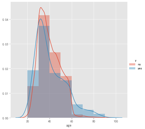
Figure 1. Age histogram.

As can be seen in Figure 1, only a small proportion of the bank's clients are under the age of 20 or below, with the age distribution concentrated in the middle-aged and young people aged 30 to 50, with an average age of 40.2 years. People in this age group have stable incomes, which may have an impact on the signing of products.

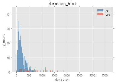
Figure 2. Duration distribution.

Customer call times who accept this deposit product are higher than that of the customer who did not accept, indicating that the variable may have a significant impact on the corresponding variable (Figure 2).

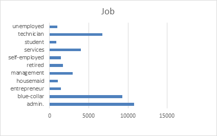
Figure 3. Job distribution.

Among the bank's customers. Executives, blue-collar workers, and technicians are in the top three, and the number of students, maids and unemployed are smaller, not to mention unknown jobs (Figure 3).

3. Methodology

The four-step methodology is used to determine purchase intent (Figure 4）

3.1. Step 1: correlation analysis

The correlation coefficient can reflect the relationship between two variables and their related directions. This can directly help us focus on some distinct highly related variables. However, the correlation coefficient cannot exactly demonstrate the relation degree between two variables. More analysis is still needed when making choices of variables.

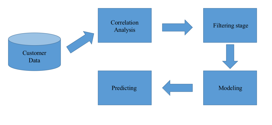
Figure 4. Methodology.

Notes: Dealing with the customer data, first of all, the correlation analysis is done to find some distinct highly related variables. Then in the filtering stage, the customer data is filtered and cleaned to conduct efficient computation. Next, in the modeling stage, the Apriori algorithm has done its job to describe the association between variables and the decision tree to learn and output the final model. Finally, in the prediction stage, customer purchase is made according to the user’s intent based on the previous results.

3.2. Step 2: filtering stage

It is widely acknowledged that there exists useless information or abnormal values in the database. Because of that, filtering and cleaning the data is necessary for efficient computation.

3.2.1. Identification of outliers. Usually, the identification of outliers can be done using graphical methods (such as box plots, normal distribution diagrams) and modeling methods (such as linear regression, clustering algorithm, K nearest neighbor algorithm). In this research, two Graphical methods and a method of identifying outliers are shared based on models.

3.2.2. Box plot. The box plot technique is used to section off quantiles of data to identify outliers. It’s a typical statistical graph and is widely used in academia and industry. The lower quantile in the figure refers to the value corresponding to the 25% quantile of the data ( \( Q1 \) ); the median is the value corresponding to the 50% quantile of the data ( \( Q2 \) ); the upper quartile is the number corresponding to the 75% quantile of the data ( \( Q3 \) ); the calculation formula for the upper whisker is \( Q3+1.5 (Q3-Q1) \) ; the calculation formula for the lower whisker is \( Q1-1.5 (Q3-Q1) \) . Among them, \( Q3-Q1 \) represents the interquartile range. If a box plot is used to identify outliers, the criterion for judging is when the data value of the variable is greater than the upper whisker of the box plot or smaller than the lower whisker of the box plot, such a data point can be considered an abnormal point. Therefore, based on the box plot above, the abnormal points and extreme abnormal points in a numerical variable can be defined, and their judgment expressions are shown in table 2:

Table 2. (Judgment expression)

Using the matplotlib module in Python to visualize data is vital, where the boxplot function is used to draw box plots. Taking the data of the number of sunspots from 1700 to 1988 as an example, the box plot method is used to identify outliers in the data (Figure 5)

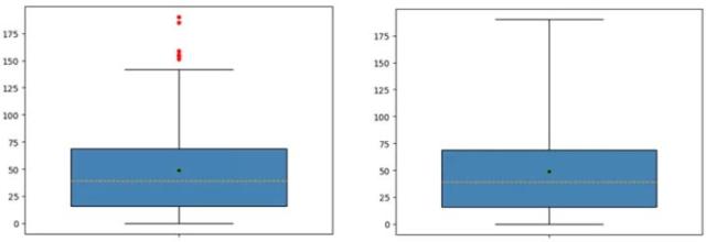
Figure 5. Example of the box plot.

Note: As shown in the figure above, the boxplot function in the matplotlib submodule plot can be used to draw box plots very conveniently. The top and bottom of the left figure must be set to 1.5 times the interquartile range, and the top and bottom of the right figure must be set to 3 times The interquartile range. It can be seen from the left image that there are at least 5 abnormal points in the data set, all of which are above the upper whiskers; however, no extreme abnormal points are shown in the right image.

3.2.3. Normal distribution diagram. According to the definition of standard normal distribution, the probability that data information points fall within 1 standard deviation (sigma value) of the average positive and negative poles is 68.2%; data information points fall within 2 relative standard deviations of the average positive and negative poles. The probability is 95.4%; the probability that the data information point falls within 3 standard deviations from the mean positive and negative is 99.6%.

Therefore, consider the probability value mentioned above from another perspective. If the probability that a data information point falls outside the two standard deviations of the average positive and negative poles is less than 5%, it is accidental, that is, that information point is considered an abnormal point. Similarly, if the data information point falls outside the three standard deviations of the average positive and negative poles, the probability will be even smaller. This kind of data information point can be regarded as an abnormal point due to extremes. In order to better let the reader, understand the probability value mentioned in the article content, the probability density graph of the standard normal distribution can be inquired, as shown in the figure below (Figure 6):

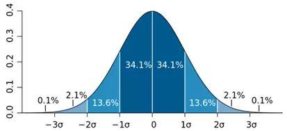
Figure 6. Probability Density diagram of the standard normal distribution.

Further, based on the conclusion of the above figure, the abnormal points and extreme abnormal points of the numerical variables can be identified according to the judgment conditions in the following table (Table 3):

Table 3. Judgment conditions.

Using the knowledge points of normal distribution, combined with the plot function in the Pyplot sub-module, draw line graphs and scatter plots, and identify outliers or extreme outliers with the help of two horizontal reference lines.

3.3. Step 3: modeling

Apriori algorithm is used to describe the association between variables, fitting the model by optimizing the Apriori algorithm, generating a combination of two or more associated variables, and then using the decision tree to learn and output the final model [12].

3.3.1. Apriori. Apriori [13] is an optimization algorithm for the discovery of current itemsets and association rules learning and training on relational databases. It is based on identifying a new item that recurs in the database query and expands them to a large new item set, as long as this new item set occurs repeatedly in the database query. As everyone knows, the Apriori optimization algorithm has two shortcomings. The first is that the number of itemsets converted into alternatives is likely to be very large. The second is the time-intensive daily task of measuring applicability. Scanner item set database query over and over [14].

Figure 7 is an example of Apriori shown below:

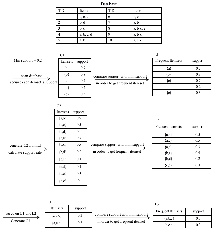
Figure 7. Example Apriori.

Note: Example of apriori algorithm flowchart.

Association rule

Association rule analysis is a technique to uncover how items are associated with each other. There are three common ways to measure association [15].

Support

This says how popular an itemset is, as measured by the proportion of transactions in which an itemset appears.

\( Support \lbrace X\rbrace = \frac{\lbrace X\rbrace }{number(all samples)} \) (1)

Confidence

This says how likely item \( Y \) is purchased when item \( X \) is purchased, expressed as \( \lbrace X - \gt Y\rbrace \) . This is measured by the proportion of transactions with item \( X \) , in which item \( Y \) also appears.

\( Confidence\lbrace X→Y\rbrace =\frac{Support\lbrace X ,Y\rbrace }{Support\lbrace X\rbrace } \) (2)

Lift up

This shows the probability of buying product \( Y \) when buying product X and at the same time manipulates product \( Y \) 's popularity level. A thrust value exceeding 1 indicates that if item \( X \) is purchased, it is likely to choose shopping item \( Y \) , while a value below 1 indicates that if item \( X \) is purchased, it is unlikely to choose shopping item \( Y \) . 

\( Lift\lbrace X→Y\rbrace =\frac{Support\lbrace X ,Y\rbrace }{Support\lbrace X\rbrace ×Support\lbrace Y\rbrace } \) (3)

Main steps

Step 1: Calculate the compatibility of the object. The combination in the query of the transaction management database ( \( size k = 1 \) ) (note that the suitability is the frequency of the occurrence of the item set). This is called transforming into a candidate set.

Step 2: Cut the alternative set according to the project whose applicability of removal is lower than the given threshold (Figure 8)

Step 3: Add a regular itemset to generate a combination of \( size k 1 \) , and repeat the above combination until no more itemsets can be generated. This situation occurs when the resulting combination has lower applicability than the given applicability [15].

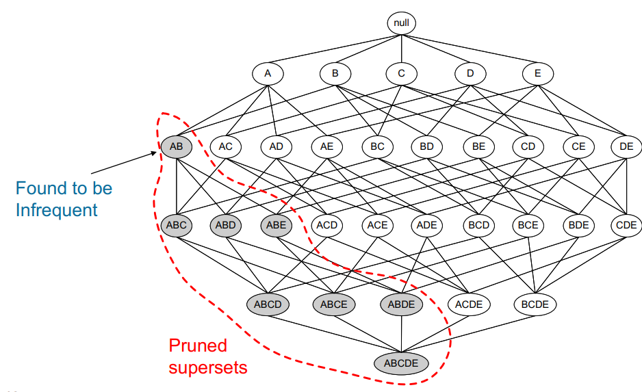
Figure 8. Apriori Pruning [10].

Note: It started from every single item in the item setlist. Then, the candidates are generated by self-joining. Extending the length of the item sets one item at a time. The subset test is performed at each stage and the item sets that contain infrequent subsets are pruned. Repeating the process until no more successful item sets can be derived from the data is very important.

3.3.2. Decision tree algorithm. The decision tree algorithm is based on the known occurrence probability of various situations. By constructing the decision tree, the probability that the expected value of the net present value is greater than or equal to zero is obtained, the project risk is evaluated, and its feasibility is judged. This is a decision analysis method that intuitively uses probability analysis. There are two main disadvantages of the decision tree algorithm: first, it is prone to overfitting. Second, the correlation of attributes in the data set is easily ignored.

After a period of development trend, various decision tree algorithms have been improved, their characteristics have been gradually improved, and they can solve various types of data information. Some major optimization algorithms will be discussed below.

ID3

The ID3 (Iterative Dichotomiser 3) algorithm is developed by Quinlan [9]. It uses information gained to select the appropriate attributes for each node of the generated decision tree. The attribute with the highest information gain (the greatest degree of entropy reduction) is used as the test attribute of the current node. In such a way, the information required to classify the subset of training samples obtained from the later division will be minimal.

CART

The classification and regression tree (CART) is proposed by Breiman et al. [14]. This is a non-parametric decision tree learning technology that generates either a classification tree or regression tree based on whether the dependent variable is categorical or numerical. It uses the Gini index for choosing attributes.

C4.5

The C4.5 algorithm is developed by Quinlan [9]. It is an improved version of the ID3 algorithm. This algorithm uses information gain as a splitting standard. It can handle missing attribute values, which is an improvement from the ID3 algorithm

Figure 9 is an example of tree algorithm shown below:

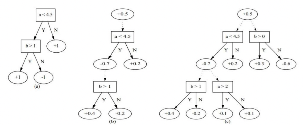
Figure 9. Example of a tree algorithm [14].

3.4. Step 4: predicting

Based on Apriori results, it can be concluded that people with certain characteristics are more likely to buy or not to buy the product. Then, using these variables to make customers' profiles predict their purchase intent is highly recommended. Next, putting the variables from Apriori into Decision Tree algorithm to process and forecast models which can also help predict customers' purchase intent [14].

4. Result

In Apriori analysis results (Table 4,5), all the lift values’ are greater than 1, which means variables are related tight with each other. Then, sorted the confidence values in descending order and pick the leading terms. It is obvious that customers who are willing to purchase the deposit products usually have the following characteristic: have no credit in fault, do not have a loan, have a housing loan, have a university degree, marital status is single, and work as an admin. On the contrary, customers who are not willing to purchase the products usually have married marital status, have no credit in fault, have no housing loan, work as blue-collar or technician, and have basic 4 or 9 education or high school degree [14].

Table 4. Apriori results (1).

Table 4. (continued).

Table 5. Apriori Results (2).

Table 5. (continued).

Then, users can use the variables from the results to create customers’ profiles (Figure 10) and put those characteristics into cloud words in order to make the results more obvious.

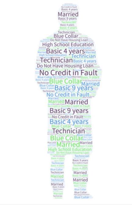
Figure 10. Cloud words of customer characters [16].

Note: The left cloud words are customers who are willing to purchase the deposit product and the right cloud words are those not willing to purchase [16].

5. Conclusion

Using apriori algorithm to create customer profiles, it can be found that customers who are willing to purchase the deposit products usually have the following characteristics: have no credit in fault, do not have a loan, have a housing loan, have a university degree, marital status is single, and work as an admin. Therefore, it can be easily concluded that in the deposit products selling, if the customers own the above characteristics, they may be more interested in the products. In other words, it will be more likely to sell the products successfully. In future work, more customer purchase information is highly needed besides the deposit products so as to extend our predictable results to a wider range.

References

[1]. Walrave, M., Poels, K., Antheunis, M.L., Van den Broeck, E., van Noort, G. (2018) Like or dislike? Adolescents’ responses to personalized social network site advertising. Journal of Marketing Communications. 24: 599-616.
[2]. Semerádová, T., Weinlich, P. (2019) Computer estimation of customer similarity with Facebook lookalikes: Advantages and disadvantages of hyper-targeting. IEEE Access. 7: 153365-153377.
[3]. Bleier, A., Eisenbeiss, M. (2015) Personalized online advertising effectiveness: The interplay of what, when, and where. Marketing Science. 34: 669-688.
[4]. Marquis, A. (n.d.) Definition of transparency advertising. https://smallbusiness.chron.com/definition-transparency-advertising-35939.html.
[5]. Felfernig, A., Jeran, M., Ninaus, G., Reinfrank, F., Reiterer, S. (2013) Toward the next generation of recommender systems: Applications and research challenges. In: Tsihrintzis, G.A., Virvou, M., Jain, L.C. (Eds.), Multimedia services in intelligent environments: Advances in recommender systems. Springer International Publishing, Heidelberg, pp. 81-98.
[6]. Burke, R. (2000) Knowledge-based recommender systems. Encyclopedia of Library and Information Systems. 69: 180–200.
[7]. Chung, R., Sundaram, D., Srinivasan, A. (2007) Integrated personal recommender systems. In: Proceedings of the ninth international conference on Electronic commerce. Minneapolis, MN, USA. pp. 65–74.
[8]. Quinlan, J.R. (1986) Induction of decision trees. Machine Learning. 1: 81-106.
[9]. Pazzani, M.J., Billsus, D. (2007) Content-based recommendation systems. In: Brusilovsky, P., Kobsa, A., Nejdl, W. (Eds.), The adaptive web: Methods and strategies of web personalization. Springer Berlin Heidelberg, Berlin, Heidelberg, pp. 325-341.
[10]. Kim, J.W., Lee, B.H., Shaw, M.J., Chang, H.-L., Nelson, M. (2001) Application of decision-tree induction techniques to personalized advertisements on internet storefronts. International Journal of Electronic Commerce. 5: 45-62.
[11]. Agrawal, Rakesh, et al.(1998) Fast Algorithms for Mining Association Rules, Fast Algorithms for Mining Association Rules and Readings in Database Systems 3rd Ed.,97-102.
[12]. Moro, S., Cortez, P., Rita, P. (2014) A data-driven approach to predict the success of bank telemarketing. Decision Support Systems. 62: 22-31.
[13]. Agrawal, R., Srikant, R., (1994). Fast algorithms for mining association rules. Proceedings of the 20th International Conference on Very Large Data Bases, Santiago, Chile, pp. 487-499.
[14]. Breiman, L., Friedman, J., Olshen, R., Stone, C. (2017) Classification and regression trees.
[15]. Chonyy. (2020) Apriori: Association rule mining in-depth. https://towardsdatascience.com/apriori-association-rule-mining-explanation-and-python-implementation-290b42afdfc6.
[16]. Freund, Y., Mason, L. (1999) The alternating decision tree learning algorithm. In: International Conference on Machine Learning. pp. 124-133.
Cite this article
Yu,R.;Li,D.;Liu,Y. (2023). Modeling of user profiles of financial products and comparison of purchase prediction models: Based on machine learning. Applied and Computational Engineering,2,64-77.
Data availability
The datasets used and/or analyzed during the current study will be available from the authors upon reasonable request.
Disclaimer/Publisher's Note
The statements, opinions and data contained in all publications are solely those of the individual author(s) and contributor(s) and not of EWA Publishing and/or the editor(s). EWA Publishing and/or the editor(s) disclaim responsibility for any injury to people or property resulting from any ideas, methods, instructions or products referred to in the content.
About volume
Volume title: Proceedings of the 4th International Conference on Computing and Data Science (CONF-CDS 2022)
© 2024 by the author(s). Licensee EWA Publishing, Oxford, UK. This article is an open access article distributed under the terms and
conditions of the Creative Commons Attribution (CC BY) license. Authors who
publish this series agree to the following terms:
1. Authors retain copyright and grant the series right of first publication with the work simultaneously licensed under a Creative Commons
Attribution License that allows others to share the work with an acknowledgment of the work's authorship and initial publication in this
series.
2. Authors are able to enter into separate, additional contractual arrangements for the non-exclusive distribution of the series's published
version of the work (e.g., post it to an institutional repository or publish it in a book), with an acknowledgment of its initial
publication in this series.
3. Authors are permitted and encouraged to post their work online (e.g., in institutional repositories or on their website) prior to and
during the submission process, as it can lead to productive exchanges, as well as earlier and greater citation of published work (See
Open access policy for details).