1. Introduction

Under the current information trend, the concept of Internet+ has completely overturned people’s past cognition, and e-commerce has emerged in such an environment. It refers to a commercial behavior based on computer network technology and centered on purchasing goods [1], which is an organic combination of traditional commerce and the Internet. The integration of the Internet and traditional industries has made many things that were once impossible possible, and people’s way of life has changed greatly with the emergence of Internet-related industries.

Online shopping is one of the most well-known and benefited e-commerce behaviors, which allows people to choose and buy goods without leaving home, greatly saving the costs of time and space. According to statistics, by the end of June 2021, the number of Internet users in China had reached 1.011 billion, among which the number of online shopping users was 812 million, accounting for 80.3% of the total number of Internet users. As the largest e-commerce transaction website in China, Taobao has nearly 500 million registered members, over 60 million daily fixed page views and 49,000 goods sold per minute. Frequent use of e-commerce platforms by users will generate massive browsing, collection, consumption and other behavior records in the background database, which all reflect their preferences and contain huge commercial value. Mining valuable information from these massive user and commodity data has become a key issue in the field of e-commerce research [2].

The increasing demand for online shopping has also greatly promoted the development of e-commerce platform. The thriving e-commerce market, making the industry competition pressure gradually increased. In order to develop more customers, businesses often attract users to consume by means of promotion on specific festivals. In 2021, the total transaction volume of Tmall Singles Day reached 540.3 billion yuan, up 8.45% year on year. Short-term promotion can indeed stimulate consumption, but it has little impact on e-commerce sales in the long run, which is also one of the reasons why the number of repeat purchase users in real e-commerce data is significantly less than the number of single purchase users, namely a large number of imbalance data samples.

The prediction of purchasing behavior of e-commerce customers refers to the real-time prediction of online customers’ purchasing tendency based on the behavior rules contained in consumers’ historical visit operation, server log, browsing record and product feedback information [3]. The development of artificial intelligence and big data technology provides strong support for the platform to predict consumer behavior. Customers’ needs can be understood from massive user behavior logs to achieve precise marketing and improve operation efficiency. While providing customers with better and more targeted service experience, the industry competitiveness is enhanced to achieve a win-win situation for users and merchants and e-commerce platforms.

In this paper, real consumer data from Tmall will be analyzed and studied. Imbalance data samples will be processed by random under-sampling and feature engineering is designed base on business logic. Machine learning models such as logistic regression, XGBoost, RandomForest are integrated using Soft-Voting and Stacking model fusion methods, and their prediction effects are compared.

2. Literature review

At present, people have done a lot of research on user behavior prediction. Pareto/NBD model (later known as SMC model) involves customer activity and is used to predict repeat purchase behavior in non-contractual setting [4]. The model assumes that the user randomly generates transactions with the merchant, and the whole process follows the Poisson distribution. Customers cannot be recalled after they are lost. Zhang Chunlian proposed the improved BG/NBD model based on SMC model, and the convenience of parameter setting and accuracy of prediction have been verified in medical shopping data [5]. In view of the underestimation of the repurchase rate and other problems in SMC model, Shu Fang et al. proposed a combination prediction model based on SMC model and HIPP model and confirmed the advantages of the combinatorial model by determining the optimal combination weights of the two through genetic algorithm [6].

RFM model is also a good method to predict users’ repurchase behavior originally applied in marketing field. Through the three indexes of Recency, Frequency and Monetary consumption [7], the characteristics of user transaction data were mined and subdivided, which has good characterization in reflecting customers’ preferences. Aiming at the problem that the model was not effective in analyzing profit, Xu Xiangbin et al. introduced the total profit attribute (P) into the RFM model to construct the RFP model, which effectively reduced the limitations of the traditional model [8]. Zhang Ning et al. combined the user-based collaborative filtering recommendation algorithm with the RFM model to make the original algorithm more efficient and accurate [9].

The above models which rely on a certain amount of expertise in economics and marketing require a lot of assumptions in advance. They are no longer applicable in the context of booming e-commerce and surging data volumes. Therefore, more scholars try to explore the prediction of user repurchase problem through the combination of massive user behavior data and machine learning algorithm. Wang Fang et al. used decision tree C4.5, RandomForest and Bayesian network algorithms to classify user income respectively. The result showed the classification effect of C4.5 algorithm was better when 10-fold cross-validation was used [10]. Zhu Xin et al. weighted and integrated logistic regression and SVM using Soft-Voting method, and obtained the best mixing mode through 3-fold cross-validation. Finally concluded that the fusion model had better prediction effect than the single model [11]. Yang Lihong et al. used fixed-length and variable-length window sliding methods to obtain more samples and features. Then verified them with logistic regression and XGBoost. Experiments proved that this method could obtain higher F1 score [12]. Zhang Bin et al. proposed an e-commerce user behavior prediction model based on deep forest to solve the problem that traditional machine learning methods needed to set a large number of hyper-parameters and have low prediction accuracy [13].

In view of the imbalance of positive and negative samples in user behavior data, Zhang Liyi et al. proposed to use SMOTE (Synthetic Minority Oversampling Technique) for sample expansion, and concluded that the imbalance dataset processed by this algorithm can effectively improve the model prediction accuracy [14]. Hu Xiaoli et al. introduced the strategy of “segmented sub-sampling” to balance the dataset repurchase and unrepurchase user samples, and used Stacking integrated model to combine multiple algorithms to predict users’ repurchase behavior. The experiment proved that this method has certain help to improve the prediction accuracy [15].

To sum up, user behavior prediction methods based on machine learning have become the mainstream of current academic research.

3. Methodology

3.1. Fusion model

The background of practical problems is varied. Through a lot of exploration, people can generalize an algorithm that is more suitable for dealing with a certain kind of problem, but no algorithm is universal. Algorithm fusion refers to the formation of a new combined model by integrating the learning results of several single algorithms, so as to improve the accuracy of algorithm [11]. Nowadays, people are constantly seeking breakthroughs in algorithm performance, generalization ability and other aspects. And such learning mode is gradually becoming popular.

The reasons why fusion algorithms usually achieve better generalization ability than single algorithms can be explained from the following three intuitive aspects [16]:

(1) From the perspective of data, only a sample set cannot provide enough information for the algorithm to pick the correct hypothesis. While many hypotheses selected by the algorithm have reached a certain precision. By integrating those better hypotheses can approach the only correct hypothesis in the space.

(2) From the perspective of algorithm, the correct hypothesis describing a sample set may not be in the hypothesis space of an algorithm. The hypothesis space can be extended to approach the correct hypothesis by integrating multiple hypotheses in it.

(3) From the perspective of computation, many algorithms only carry out local searches in the hypothesis space, which means that they may miss the optimal hypothesis and “trapped” in local extremums. Each single algorithm in the fusion algorithm searches from different starting points to better approximate the optimal hypothesis.

There are multiple ways to do algorithms fusion. Different algorithm fusion methods have different help to improve the final model effect. This paper focuses on comparing Soft-Voting and Stacking algorithms fusion methods.

3.1.1. Soft-Voting. The Soft-Voting model calculate mean of the probability that each individual model classifies each class. And then, the final prediction category is selected by comparing the mean value. Table 1 briefly shows the basic logic of this approach.

Table 1. How Soft-Voting works.

Assuming that Soft-Voting Classifier is the fusion of Classifier1 and Classifier2. The output probability of Classifier 1 and 2 for class A is 0.4 and 0.7, respectively. So the probability of class A finally obtained by the Soft-Voting Classifier is the average of the two, that is, (0.4+0.7) /2 = 0.55. Similarly, for class B, the probability is 0.45. In the end, the output result of fusion model is class A with highest probability.

3.1.2. Stacking. Stacking is a well-known way of classifier ensemble, which is obtained by combining multiple base-models and a meta-model [17]. Each base-learner can be homologous or heterologous. Using heterologous models is more possible to combine the advantages of different models to achieve better prediction effect.

Suppose there are N base-models. For each base model, use cross-validation and “stacked” the result to form a list of new features with the same length as the original training data. After N rounds, the new features produced by the cross-validation of each model are joined together, and the matrix obtained is regarded as the new training set. The initial label is used as the label of this training, and they are used to train the meta-model. Finally, put the results from N times test set fitting into the second layer algorithm (the meta-model) to obtain the final prediction result. The Stacking model principle is shown in Fig.1.

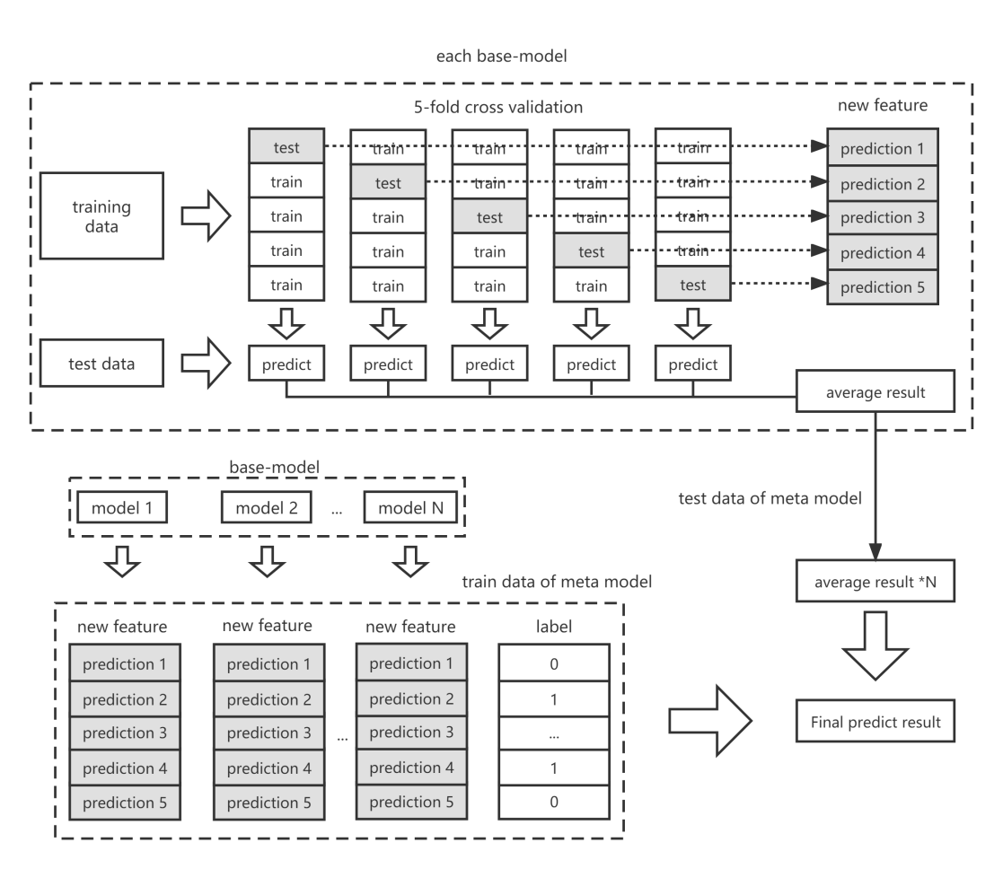
Figure 1. Structure diagram of the 5-fold cross-validation Stacking integrated model.

3.2. Model algorithm

3.2.1. Logistics regression. In order to deal with the classification problem, logistic regression combines Sigmoid function on the basis of linear regression, making the value mapping of linear regression between 0 and 1. The Sigmoid function takes 0.5 as the threshold value. If the value is higher than this value, the sample will be judged as 1, and if it is lower than this value, it will be judged as 0. Sigmoid function expression and its diagram are as follows.

\( y =\frac{1}{1+{e^{-z}}} \) (1)

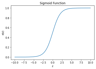
Figure 2. Schematic diagram of Sigmoid function.

The linear regression model formula is:

\( z = {w^{T}}x+b \) (2)

Substitute formula (2) to obtain the model expression of the logistic regression:

\( ln\frac{y}{1-y} = {w^{T}}x+b \) (3)

Given the training set \( \lbrace ({x_{i}}, {y_{i}})\rbrace _{i=1}^{m} \) , if we regard \( y \) as a posterior probability \( p(y=1|x) \) of class, that is, the probability of class 1 under sample \( x \) conditions, then:

\( ln\frac{p(y=1|x)}{p(y=0|x)} = {w^{T}}x+b \) (4)

Then, the cross entropy loss function is:

\( lnp(y|x) = ylnŷ+(1-y)ln(1-ŷ) \) (5)

where,

\( ŷ=\frac{1}{1+{e^{-({w^{T}}x+b)}}} \) (6)

Let \( L=lnp(y|x) \) , take the partial derivatives of \( w \) and \( b \) based on \( L \) :

\( \frac{∂L}{∂w} =\frac{1}{m}x(ŷ-y) \) (7)

\( \frac{∂L}{∂b} =\frac{1}{m}\sum _{i=1}^{m}(ŷ-y) \) (8)

Then gradient descent based on \( w \) and \( b \) minimizes the cross entropy loss, the corresponding parameters are the optimal parameters of the model.

3.2.2. KNN. KNN is known as k-nearest neighbor machine learning model. It is considered one of the simplest algorithms, but very effective. For a given test sample, the algorithm will find k training samples closest to the training set according to some distance measure. And then it makes a prediction based on the k neighbors [18].

It is a classic representative of lazy learning, because it has no explicit training process. The training time complexity of this KNN is 0, in other word, KNN does not need to use the training set for training and only processes the test data after receiving it.

The above contents can be summarized as the following three important factors affecting the k-nearest neighbor prediction effect:

Distance Calculation Method. KNN algorithm uses distance to measure the similarity between two samples. The commonly used distance representation methods include “Minkowski Distance”, “Manhattan Distance” and “Euclidean Distance”. The Euclidean Distance equation is as follow:

\( D(x, y) = \sqrt[]{\sum _{i = 1}^{n}{({x_{i}}-{y_{i}})^{2}}} \) (9)

The Value of k. The choice of k value should be moderate. When the value of k is small, the training error decreases relatively, but the model complexity becomes high, and the problem of overfitting is easy to occur. A larger k value means that more remote (less similar) samples are selected to participate in the prediction, which will lead to increased training error and reduced model complexity.

Decision Making. For classification tasks, k-nearest neighbor algorithm usually uses “voting method” or known as “majority voting method” to make decisions, that is, the output result is the majority class among k training samples. We can also assign weights based on the distance between the testing sample and the training sample. The closer the sample is, the greater the similarity is and the greater the weight is.

We define the training error rate as the proportion of k-nearest neighbor training samples whose labels are inconsistent with the input labels. Given the test sample \( x \) , if its nearest neighbor sample is \( z \) , then the error rate of the classifier is the probability that the class of \( x \) and \( z \) are labeled differently, which is expressed as:

\( P(err) =1 -\sum _{c∈y}P(c|x)P(c|z) \) (10)

The schematic diagram of the 3 nearest neighbor model [19] is shown in Fig.3.

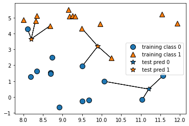
Figure 3. Prediction results of forge dataset by 3-nearest neighbor model.

For the input test sample, select the 3 nearest training set data samples around it and take a vote. The test sample will be judged as the majority class in the vote.

3.2.3. RandomForest. RandomForest (RF) is an integrated learning algorithm based on Bagging framework proposed by Breiman in 2001 [20]. It is composed of CART decision tree based classifier. Assuming that the data has M samples and N features, the construction principle of RandomForest is as follows:

(1) Select M samples with replacement.

(2) When each node that makes the decision needs to be split, pick a random subset of K features from these N features (K<<N and generally choose K=log2N). Then select features from the K features for node splitting, which increases the “diversity” of both samples and features.

(3) Each node is split according to step (2) until it cannot be split.

(4) A large number of decision trees are constructed to form a RandomForest by repeating the above steps. For classification problems, the result of each tree is voted to get the final output.

Therefore, the randomness of RandomForest can be summarized as the “randomness of training samples” of each tree and the “randomness of node splitting attributes” of each tree. Also thanks to these two “randomness”, random forest is not easy to have over-fitting situation.

3.2.4. XGBoost. XGBoost is short for extreme Gradient Boosting. It optimizes the GBDT algorithm and uses multiple CART decision trees to provide the accuracy of the prediction model. And then, the prediction results of the decision tree obtained in each round of training are summed to obtain the final predicted value [21].

From the perspective of algorithm accuracy, XGBoost can better approximate the real loss by expanding the loss function to the second derivative. From the perspective of the generalization ability of the algorithm, XGBoost adds regularization term to the loss function which can prevent the model from overfitting. Assuming that the data contains \( n \) samples and \( m \) features:

\( D = \lbrace {(x_{i}}, {y_{i}})\rbrace (|D| = n, {x_{i}}∈{R^{m}}, {y_{i}}∈R) \) (11)

XGBoost will train multiple trees in the process of forward iteration and further reduce the prediction error by combining the prediction results of the previous tree.

\( {ŷ_{i}} = \sum _{k = 1}^{K}{f_{k}}({x_{i}}) , {f_{k}}∈F \) (12)

where \( F = \lbrace f(x) = {w_{q(x)}}\rbrace (q:{R^{m}}→T, w∈{R^{T}}) \) , which is the set of all possible CART decision trees. \( T \) is the number of leaf nodes in each tree, \( w \) is the weight of leaf nodes in each tree, \( γ \) and \( λ \) are the coefficients. \( {f_{k}} \) is the k-th independent CART tree, and K is the total number of CART trees.

The original objective function consists of empirical loss term and regularization term:

\( L(∅) = \sum _{i}l({y_{i}} , {ŷ_{i}})+ \sum _{k}Ω({f_{k}}) \) (13)

where \( l({y_{i}} , {ŷ_{i}}) \) is the loss function of the model, which represents the difference between the prediction \( {ŷ_{i}} \) and the true value \( {y_{i}} \) ; the term \( Ω({f_{k}}) \) penalizes the complexity of the model [21], this is how XGBoost controls overfitting accordingly.

Put all samples \( {x_{i}} \) belonging to the j-th leaf node into the sample set of a leaf node, that is \( {I_{j}} = \lbrace i|q({x_{i}})=j\rbrace \) . So the model complexity can be expressed as:

\( Ω(f)=γT+\frac{1}{2}λ{‖w‖^{2}}= γT + \frac{1}{2}λ\sum _{j = 1}^{T}w_{j}^{2} \) (14)

According to the forward distribution algorithm, the objective function after the t-th iteration can be written as:

\( {L^{(t)}} = \sum _{i = 1}^{n}l({y_{i}} , ŷ_{i}^{(t-1)}+{f_{t}}({x_{i}})) +Ω({f_{t}}) \) (15)

where \( {{ŷ_{i}} ^{(t)}} \) is the prediction of the i-th instance at the t-th iteration.

Using the second-order Taylor expansion for formula (15) and removing the constant term, the objective function can be simplified as:

\( {L^{(t)}} = \sum _{i=1}^{n}[{g_{i}}{f_{t}}({x_{i}})+\frac{1}{2}{h_{i}}f_{t}^{2}({x_{i}})] +Ω({f_{t}}) \) (16)

where \( {g_{i}} \) , \( {h_{i}} \) are first and second order gradient statistics on the loss function:

\( {g_{i}} = {∂_{ŷ_{i}^{(t-1)}}}l({y_{i}} , ŷ_{i}^{(t-1)}) \) (17)

\( {h_{i}} = ∂_{ŷ_{i}^{(t-1)}}^{2}l({y_{i}} , ŷ_{i}^{(t-1)}) \) (18)

After substituting formula (14) into formula (16), the objective function can be simplified as:

\( {L^{(t)}} = \sum _{j=1}^{T}[{G_{j}}{w_{j}}+\frac{1}{2}{{({H_{j}}+λ)w_{j}}^{2}}] +γT \) (19)

where, \( {G_{j}} \) and \( {H_{j}} \) are the sum of the first and second partial derivatives of the samples contained in leaf node \( j \) . They are:

\( {G_{j}}=\sum _{i∈{I_{j}}}{g_{i}} \) (20)

\( {H_{j}}=\sum _{i∈{I_{j}}}{h_{i}} \) (21)

Taking the derivative of Formula (19), the optimum point and optimal value of leaf node \( j \) are respectively:

\( w_{j}^{*} = -\frac{{G_{j}}}{{H_{j}}+λ} \) (22)

\( {L^{(t)}} = -\frac{1}{2}\sum _{j=1}^{T}\frac{{{G_{j}}^{2}}}{{H_{j}}+λ} +γT \) (23)

4. Result

4.1. Experimental data

The data is the real user behavior data of Tmall which comes from the Tianchi Competition platform. It mainly consists of user behavior log data and user profile data.

4.1.1. User behaviour log data. As shown in Table 2, the user behavior log data records the types of user actions in the merchant, the time when those actions occurred as well as the corresponding item, item category and item brand.

Table 2. User behavior log data.

4.1.2. User characteristic data. As shown in Table 3, the user characteristic data summarizes the age range and gender of each visiting user and whether they have repeated purchase behaviors.

Table 3. User characteristic data.

4.2. Data preprocessing

Raw data collected in the real world often varies a lot in both quality and type. Therefore, the process of data mining is particularly important in the process of machine learning. How to effectively process data and create features can help the

model and algorithm approach the upper limit of its prediction, and better help enterprises to discover valuable users.

4.2.1. Null values. In real business scenarios, errors or missing values are commonly seen during data collection. For the user behavior log data and user characteristic data, only “brand_id” contains 91,015 null values. To ensure sample integrity, “0” is used for supplementary processing.

4.2.2. Sample equalization. There are 260,864 samples data in total, including 244,912 negative samples (users labeled as 0) and 15,952 positive samples (users labeled as 1). The proportion of positive samples is 6.115%, which means this is a serious imbalance data of positive and negative samples, as shown in Fig.4.

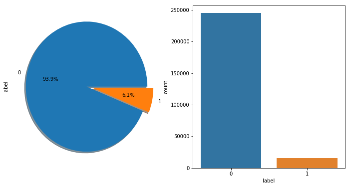
Figure 4. Percentage of positive and negative data samples before sampling.

If we input imbalance sample data into the classifiers, the results of them are more likely be affected by the majority class samples, leading to a serious decline in the prediction effect. The mainstream methods of dealing with imbalance data are oversampling represented by SMOTE [22], and under-sampling.

In order to save computer memory resources and improve operation efficiency. All the positive samples with great learning value are reserved, and then the negative samples are reduced using random under-sampling. The total amount of data after sampling is 31,904, including 15,952 negative samples and 15,952 positive samples. The ratio of positive and negative samples is 1:1.

4.3. Feature engineering

Feature engineering refers to mining excellent features for model training from a large amount of data. This paper constructs 50 data features from 3 aspects, that is, “user features”, “merchant features” and “user-merchant features”. As shown in Table 4.

Table 4. Features explanation table.

4.4. Model parameter

Both Soft-Voting and Stacking model integrate the prediction results of multiple individual models to finish the prediction. In this experiment, GridSearchCV is used in adjusting the performance of each model to a better state.

The essence of GridSearchCV is to use grid search with cross-validation to adjust parameters. It combines the values of each candidate parameter in turn, and then determines the optimal model parameters by using the results of cross-validation. However, the exhaustive process of grid search tends to increase the computational complexity, making the parameter adjusting process quite long. Therefore, several parameters that have greater influence on the results of each algorithm are selected in the parameter adjustment.

Furthermore, stratified k-fold cross-validation is used for parameter adjustment. In stratified k-fold cross-validation, the ratio between classes in each fold is the same as the ratio in the entire datasets [19]. It can effectively avoid the situation that one fold only contains the majority class samples when dividing imbalance datasets. This helps to make a more reliable estimate of model generalization performance. In this experiment the stratified 5-fold cross-validation is chosen. The principle of this method [19] is shown in Fig.5.

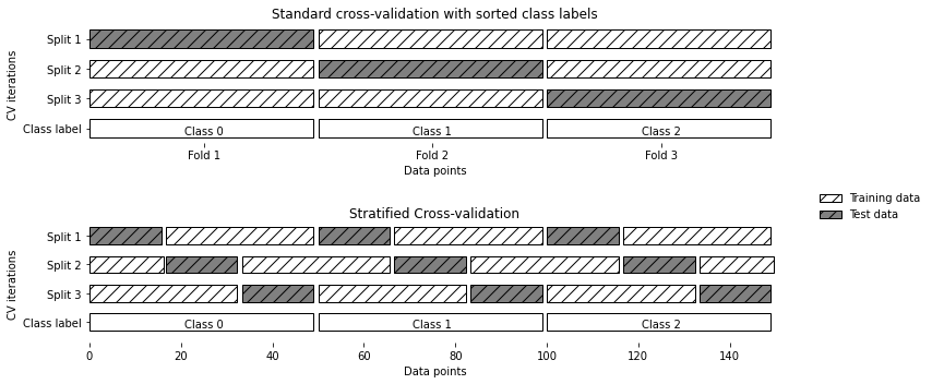
Figure 5. Schematic diagram of stratified k-fold cross-validation.

After adjusting the main parameters of each model, the parameter values are as shown in Table 5.

Table 5. The Chosen model parameters after stratified 5-fold cross-validation.

4.5. Model building

In this paper, Soft-Voting and Stacking are used for comparative analysis. In order to enhance the accuracy and generalization performance after model fusion, several heterogeneous algorithms are selected for combination, including logistic regression, k-nearest neighbor, XGBoost and RandomForest.

Soft-voting model averages the predicted results of the four base-models and assigns weights based on the predicted results of each of them. The established Soft-Voting model is shown in Fig.6.

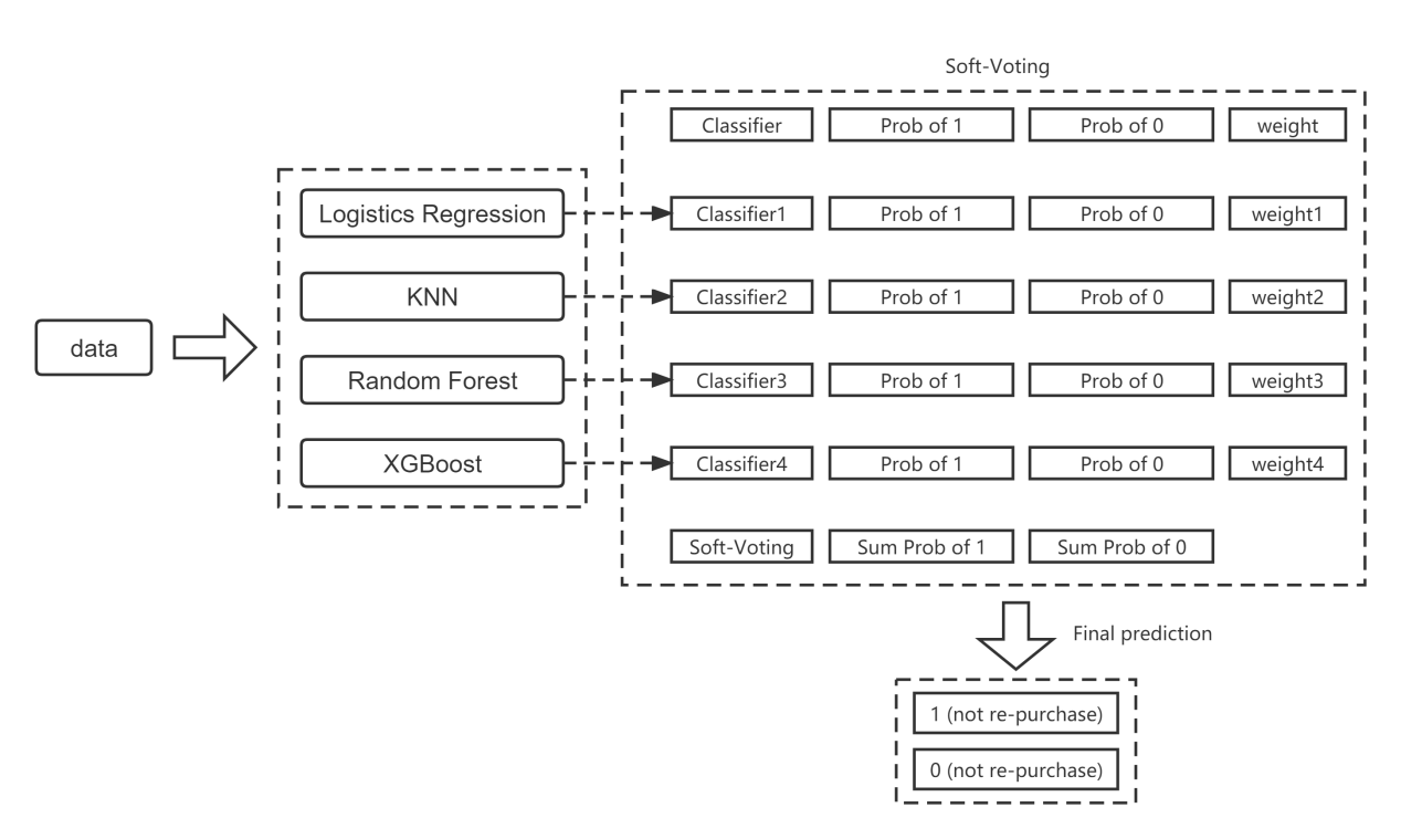
Figure 6. Soft-Voting model diagram.

Stacking model has two layers. In this experiment, k-nearest neighbor, XGBoost and RandomForest were used in the first layer. And a relatively simple algorithm is generally used in the second layer to prevent overfitting situation. This time logistic regression is used. The established Stacking model is shown in Fig.7.

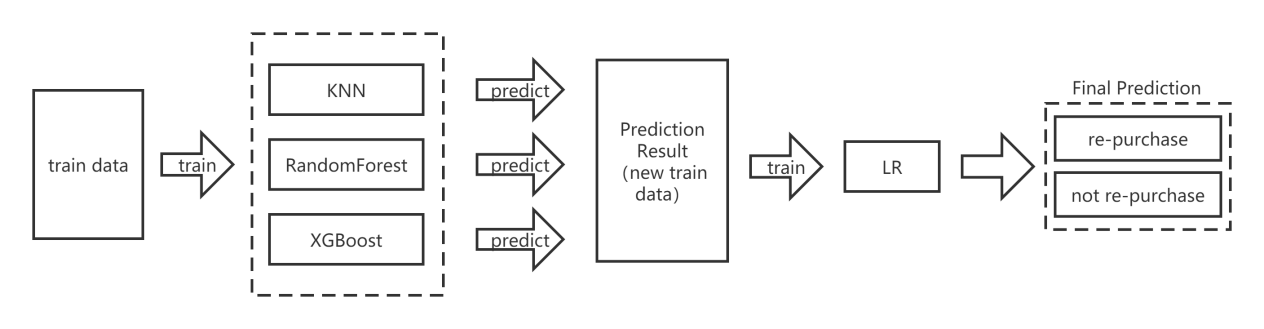
Figure 7. Stacking model diagram.

4.6. Experiment result

4.6.1. Evaluation method. As is known that there are two classes in binary classification, positive and negative. So, according to the real class in the sample and the predicted class of the model, there will be four cases: true positive (TP), false positive (FP), true negative (TN) and false negative (FN).

In this experiment, TP and TN respectively represent the number of repurchased and unrepurchased samples correctly predicted by the model. FP and FN respectively represent the number of repurchased and unrepurchased samples incorrectly predicted by the model.

Receiver Operating Characteristics Curve is referred to as ROC Curve. The ROC curve shows the true positive rate (TPR) and false positive rate (FPR), which can directly reflect the sensitivity and accuracy of the model when selecting different thresholds [23]. The two formulas are as follows:

\( TPR = \frac{TP}{TP+FN} \) (24)

\( FPR = \frac{FP}{FP+TN} \) (25)

Area Under Curve (AUC) refers to the Area enclosed by the ROC Curve and the coordinate axis, which can more intuitively reflect the effect of the model. In other words, AUC can be understood as the probability that positive samples selected by classifier is ranked before negative samples, and its formula is as follow:

\( AUC = \frac{\int _{0}^{1}TP dFP}{(TP+FN)+(TN+FP)} \) (26)

The value of AUC ranges from 0.5 to 1. The closer the AUC value of the model is to 1, the higher its practical application value is.

4.6.2. Experiment result. Based on the datasets, constructed features and model parameters. The output prediction results of Soft-Voting, Stacking fusion models and individual classification model are shown in Table 6.

Table 6. Comparison of output results of each classification model.

5. Discussion

In this experiment, k-nearest neighbor, RandomForest, XGBoost and logistic regression were used for individual model prediction. As can be seen from the experimental results in the table, the AUC values predicted by XGBoost, random forest, logistic regression and KNN decrease successively. The difference between RandomForest and XGBoost algorithm in AUC value is small, while XGBoost is better. Because XGBoost model is optimized by adding loss function and regularization strategy based on GBDT, it can effectively prevent overfitting and improve accuracy. However, KNN algorithm belongs to “lazy learning” and there is no strict training process. Compared with other more complex algorithms, its AUC value is lower.

For both Soft-Voting and Stacking fusion models, the AUC values are higher than those of the four individual algorithms. Soft-Voting model improved significantly after it is weighted, with the AUC value rising from 0.6656 to 0.6681. It can be concluded that weighting helps greatly in accuracy improvement.

The AUC value of the Stacking model reached 0.6679, which is similar to the AUC of Soft-Voting model. Because multiple heterogeneous algorithms in the first layer of Stacking can collaborate to learn the features of the input data more effectively, reducing the error rate of model classification. In combination with the second layer, the prediction performance of the fusion model can be further improved.

It can be clearly seen that the time cost of fusion model training is higher, which is an inevitable cost in the process of increasing the complexity of the model. The training time of weighted Soft-Voting method is slightly longer due to the weighting process. The Stacking method has its built in 5-fold cross-validation, resulting in much higher training time than other models.

6. Conclusion

This paper compares the two fusion methods in the same e-commerce repurchase prediction scenario. The final AUC value of the fusion model is significantly improved than that of the single model.

The Stacking method uses a two-layer prediction structure. The output of the first layer prediction is packed into a new training set for the second layer model, which increases the computational complexity and takes longer training time, but also gets higher AUC value.

The Soft-Voting method generates new results by adding and averaging the predicted results of individual models, and requires more detailed model weighting process to achieve better results. For future experiments, the following directions can be considered:

(1) More complex models, such as SVM, can be considered in the selection of a base-model to replace less effective models in this experiment.

(2) Both Stacking and Soft-Voting rely on the fusion of multiple models. The diversity of models can improve the prediction effect to some extent, but the model generalization performance and fitting may be affected. A better combination and weighting method needs to be further discussed.

(3) In the aspect of feature engineering, more complex and multidimensional features can be considered.

(4) The under-sampling method will lose important learning information to some extent. Data sampling methods, such as SMOTE, can be considered to keep as many samples as possible to improve learning results.

References

[1]. Wang B Y. The Study on the Industrial Evolution,Competitive Situation and Development Trend of Chinese Online Retail Industry[J]. China Business and Market, 31(4):25-34 (2017).
[2]. Wang Y, Ruan M L. Risk Estimation Simulation of Excess Trading Transactions Based on Big Data[J]. Computer Simulation, 35(3):369-372 (2018).
[3]. Yang G S, Guo B B. User Behavior Prediction for E-commerce Platforms Enhanced by Machine Learning[J]. Science and Technology & Innovation, 2019
[4]. Schmittlein D C, Morrison D G, Colombo R. Counting Your Customers: Who are They and What will They Do Next? [J]. Management Science, 33(1): 1-24 (1987).
[5]. Zhang C L. Research on BG/NBD Prediction Model and Its Application of the Customer Purchase Behavior[D]. Harbin Institute of Technology, 2006.
[6]. Shu F, Ma S H. A Composition Forecasting Approach of Customer Repeat Purchasing[J]. Computer and Modernization,2015(5):67-70 (2015).
[7]. Hughes A M. Boosting Response with RFM[J]. Marketing Tools, 1996, 3(3): 4.
[8]. Xu X B, Wang J Q, TU Huan, et al. Customer classification of E-commerce based on improved RFM model[J]. Journal of Computer Application, 2012, 32(5):1439-1442.
[9]. Zhang N, Fan C R, Zhang Y. A Novel Personalized Recommendation Algorithm of Collaborative Filtering Based on RFM Model[J]. Telecommunications Science, 31(9):110-118 (2015).
[10]. Wang F, Shen G C. Machine Learning Algorithms in the Application of user Behavior[J]. Computer Knowledge and Technology, 2017(26): 180 -182.
[11]. Zhu X, Liu X M, Chen S G, et al. Research on Network Purchase Behavior Prediction Based on Machine Learning[J]. Statistics & Information Forum, 2017, 32(12): 94-100.
[12]. Yang L H, Bai Z Q. User behavior prediction based on feature engineering of quadratic combination and XGBoost model[J]. Science Technology and Engineering, 18(14):186—189 (2018)
[13]. Zhang B, Fu Y, Zhou J, et al. User behavior prediction method of E-commerce platform based on deep forest[J]. Information Technology, 2021(6): 96-101.
[14]. Zhang L Y, Li Y R, Wen X. Predicting Repeat Purchase Intention of New Consumers[J]. Data Analysis and Knowledge Discovery, 2018, 2(11): 10-18.
[15]. Hu X L, Zhang H B, Dong Junchao, et al. Prediction of ensemble learning⁃based new users’ repurchase behavior on e⁃commerce platform[J]. Modern Electronics Technique, 43(11):115-119 (2020).
[16]. ZhouZH. Ensemble Learning[J]. Encyclopedia of Biometrics, 2009.
[17]. Wolpert D H. Stacked generalization[J]. Neural networks, 1992, 5(2): 241-2 59.
[18]. Zhou Z H. Machine Learning (Version I) [M]. Beijing: Tsinghua University publishing house co., ltd, 2016.
[19]. Andreas C. Müller, Sarah Guido. Introduction to Machine Learning with Python[M]. The People’s Posts and Telecommunications Press, 2018.
[20]. Breiman L, Breiman L, Cutler R A.Random Forests Machine Learning[J]. Journal of Clinical Microbiology, 2001, 2: 199-228.
[21]. Chen T, Guestrin C.Xgboost: A scalable tree boosting system[C]. San Francisco: the 22nd ACM SIGKDD International Conference on Knowledge Discovery and Data Mining, 2016: 785-794.
[22]. Chawla N V, Bowyer K W, Hall L O, et al. SMOTE: Synthetic minority over-sampling technique[J]. Journal of Artificial Intelligence Research, 2022, 16:321 - 357.
[23]. Fawcett T.ROC Graphs: Notes and practical considerations for data mining researchers[J]. Pattern Recognition Letters, 31(8): 1-38 (2003).
Cite this article
Yuwei,J. (2023). Research on prediction of e-commerce repurchase behavior based on multiple fusion models. Applied and Computational Engineering,2,90-104.
Data availability
The datasets used and/or analyzed during the current study will be available from the authors upon reasonable request.
Disclaimer/Publisher's Note
The statements, opinions and data contained in all publications are solely those of the individual author(s) and contributor(s) and not of EWA Publishing and/or the editor(s). EWA Publishing and/or the editor(s) disclaim responsibility for any injury to people or property resulting from any ideas, methods, instructions or products referred to in the content.
About volume
Volume title: Proceedings of the 4th International Conference on Computing and Data Science (CONF-CDS 2022)
© 2024 by the author(s). Licensee EWA Publishing, Oxford, UK. This article is an open access article distributed under the terms and
conditions of the Creative Commons Attribution (CC BY) license. Authors who
publish this series agree to the following terms:
1. Authors retain copyright and grant the series right of first publication with the work simultaneously licensed under a Creative Commons
Attribution License that allows others to share the work with an acknowledgment of the work's authorship and initial publication in this
series.
2. Authors are able to enter into separate, additional contractual arrangements for the non-exclusive distribution of the series's published
version of the work (e.g., post it to an institutional repository or publish it in a book), with an acknowledgment of its initial
publication in this series.
3. Authors are permitted and encouraged to post their work online (e.g., in institutional repositories or on their website) prior to and
during the submission process, as it can lead to productive exchanges, as well as earlier and greater citation of published work (See
Open access policy for details).