1. Introduction

The urgency of mitigating greenhouse-gas emissions has focused attention on electrified transport. Transportation accounted for about 28% of U.S. greenhouse-gas emissions in 2022, making it the largest contributor [1]. Because EVs have zero tailpipe emissions, broader adoption can materially lower CO₂; global scenarios project savings on the order of hundreds of millions of tons if current policy pledges are realized [2]. Many governments therefore deploy financial incentives to accelerate adoption; for example, Germany’s federal program led to a 250% increase in subsidized EV purchases between 2020 and 2021 and delivered CO₂ savings of roughly 3 million tons [3]. Similar incentive effects have been documented in China [4].

Prior work highlights income and charging access as central drivers. Studies report higher adoption with higher income [5] and emphasize that insufficient public charging can impede market growth [6]. Within King County, Washington, underinvestment in lower-income areas aligns with lower adoption [7]. Consistent with this literature, the present analysis finds positive correlations between income, charging-station availability, and EV adoption trends.

A common limitation in the literature is spatial aggregation. Analyses at the state or county level can mask local heterogeneity; coarser geographies introduce aggregation error relative to more granular units [8]. ZIP-code–level analysis can therefore reveal patterns that broader unit’s obscure.

This study assembles a 2020–2025 ZIP-code–level dataset for Washington State and estimates multivariable linear regressions linking EV adoption to urbanization, per-capita personal income, educational attainment, charger access, and family size. The analysis documents (i) positive associations with income, education, urbanization, the number of newly built local (0–20 miles) charging stations, and family size; and (ii) a negative association with the number of newly built distant (≥30 miles) charging stations, consistent with rurality effects. These results underscore the localized nature of EV adoption and inform targeted infrastructure and incentive design.

The remainder of the report is organized as follows. Section 2 describes data sources, cleaning, feature engineering, and merging. Section 3 details model selection, variable screening, and assumption checks. Section 4 presents conclusions. Section 5 discusses limitations and future directions. Section 6 lists references.

2. Data

2.1. Data acquisition and visualization

All data were harmonized to the ZIP‑code level for Washington State over 2020–2025. Vehicle registration transactions were obtained from data.wa.gov; ZIP‑code geometry and coordinates from SimpleMaps; income, population, age, and household characteristics from NHGIS; urban/rural status from data.census.gov; and public charging‑station information from the U.S. DOE Alternative Fuels Data Center (AFDC). In total, twelve datasets were assembled, several exceeding 30 million records. After standardizing identifiers and geographic keys, exploratory data analysis (EDA) guided variable selection and model design.

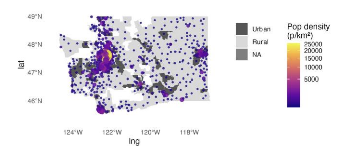
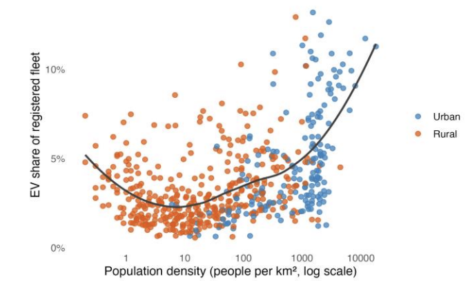
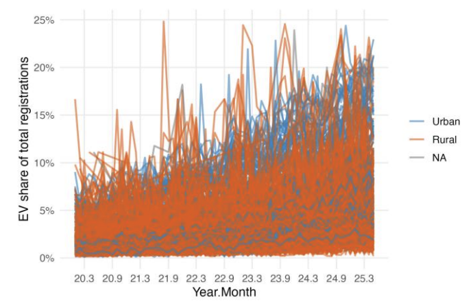
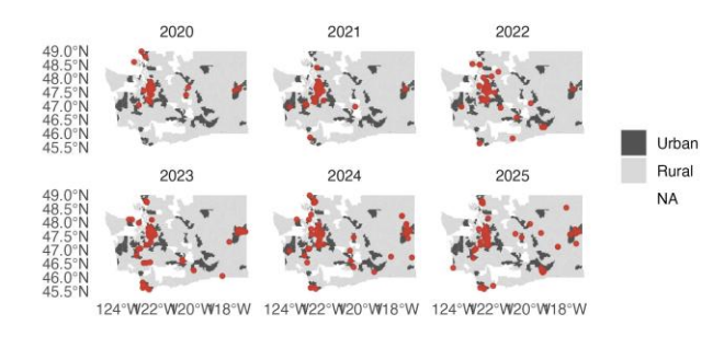
Figure 1 illustrates the strong right‑skew in population density, with urban ZIPs anchoring the upper tail. Figure 2 depicts a clear positive association between population density and the share of EVs among registered vehicles, especially apparent once urban ZIPs are highlighted. Figure 3 documents a persistent five‑year uptrend in EV adoption, with urban areas leading as early adopters. Figure 4 maps the annual rollout of charging stations, showing concentration in urban areas with gradual penetration into rural regions.

2.2. Data pre-processing

Data pre‑processing ensured internal consistency, reproducibility, and tractable model size. Procedures addressed missing data, exclusion rules for outliers and unreliable observations, feature engineering, and final merging.

2.2.1. Handling missing values

One of the primary concerns in any dataset is the presence of missing values, and complete datasets were required in the regression analysis. To address this issue, missing values were assessed before and after merging. Prior to merging, ZIPs with extensive missing fields—rare and concentrated in very sparsely populated areas with multiple unreliable statistics—were removed to avoid undue influence from noisy observations. After merging, mean imputation was applied to education proportions when necessary, using the statewide ZIP mean; imputed ZIPs constituted less than 10% of the analytic sample. This approach preserves coverage while acknowledging a potential attenuation of estimated effects, discussed in the discussion part.

2.2.2. Outliers and exclusions

EDA (boxplots and scatterplots) revealed a small number of manifest anomalies. To reduce spurious leverage, observations (ZIPs) were excluded when cumulative registrations over 2020–2025 were below 1,000, when the EV share exceeded 24.9% (implausible for the period), when average family size exceeded 10 (indicative of data error), or when the outcome construction (Section 2.2.3) yielded a non‑significant trend (slope p‑value > 0.05). Thresholds were set ex ante based on distributional evidence; sensitivity to alternative cutoffs is reported elsewhere.

2.2.3. Feature engineering

Categorical variables were encoded numerically and, where appropriate, regrouped to mitigate multicollinearity. The outcome variable is the monthly trend in EV share at the ZIP level. For each ZIP  $$ i$$ , a monthly EV‑share series (EV registrations divided by total registrations) was constructed and the following OLS was estimated (Eq. Equation 1):

$EVShar{e}_{it}={\alpha }_i+{\beta }_{i}t+{\epsilon }_{it}\mathrm{.}$(1)

The slope  $$ {\beta }_i$$  (percentage points per month) is retained when statistically significant at  $$ p\le 0.05$$ .

Education composition was expressed as ZIP‑level percentages grouped into mid‑low (≤ high school), mid‑high (high school to some college), and high (≥ college), with the very‑low category suppressed to limit collinearity. Age composition was expressed as ZIP‑level percentages for the bands 1–20, 21–30, …, 71–80, with ages ≥81 suppressed for the same reason. Urbanization was encoded as a binary indicator (Urban.Rural = 1 for urban, 0 for rural). Charging‑infrastructure access was measured as the number of new public charging stations relative to the ZIP centroid in fixed distance bands of 0–10, 10–20, 20–30, and ≥30 miles (num_0_10, num_10_20, num_20_30, num_30_plus). Distances were computed as great‑circle distances from ZIP centroids; with fixed radii, counts are directly interpretable, and density‑based normalizations are examined in robustness checks.

2.2.4. Final analysis dataset

The final merged dataset comprises the following variables: the ZIP identifier; population density (people per km²); per‑capita personal income (USD); education shares (edu_midlow, edu_midhigh, edu_high); age‑band shares from 1–20 through 71–80; an urbanization indicator (Urban.Rural, with 1 denoting urban); counts of new charging stations within 0–10, 10–20, 20–30, and ≥30 miles (num_0_10, num_10_20, num_20_30, num_30_plus); average family size (people); and the outcome slope (percentage‑point change in EV share per month). Table 1 provides concise definitions and units.

3. Methods

3.1. Model building

The empirical strategy proceeds from a saturated linear specification to progressively more parsimonious models, with formal tests at each step. Let the dependent variable be the monthly change in EV share at the ZIP level (Section 2.2.3). The initial (“full”) model, M1, includes socioeconomic composition, urbanization, and charging‑access measures:

$$$ \begin{array}{cccc}\text{slope}& & & =-4.295\times {10}^{-4}\\ & +7.130\times {10}^{-9}\hspace{0.17em}\text{population\_density}& & +8.130\times {10}^{-9}\hspace{0.17em}\text{PCPIE}\\ & +7.990\times {10}^{-5}\hspace{0.17em}\text{edu\_midlow}& & +5.448\times {10}^{-5}\hspace{0.17em}\text{edu\_midhigh}\\ & +1.313\times {10}^{-3}\hspace{0.17em}\text{edu\_high}& & -7.058\times {10}^{-4}\hspace{0.17em}\text{age\_1\_20}\\ & -5.184\times {10}^{-4}\hspace{0.17em}\text{age\_21\_30}& & +7.083\times {10}^{-4}\hspace{0.17em}\text{age\_31\_40}\\ & +8.928\times {10}^{-4}\hspace{0.17em}\text{age\_41\_50}& & +1.854\times {10}^{-4}\hspace{0.17em}\text{age\_51\_60}\\ & -4.113\times {10}^{-4}\hspace{0.17em}\text{age\_61\_70}& & +8.954\times {10}^{-5}\hspace{0.17em}\text{age\_71\_80}\\ & +6.657\times {10}^{-5}\hspace{0.17em}\text{Urban.Rural}& & +2.628\times {10}^{-7}\hspace{0.17em}\text{num\_0\_10}\\ & +3.531\times {10}^{-7}\hspace{0.17em}\text{num\_10\_20}& & +5.221\times {10}^{-8}\hspace{0.17em}\text{num\_20\_30}\\ & -3.780\times {10}^{-8}\hspace{0.17em}\text{num\_30\_plus}& & +1.315\times {10}^{-4}\hspace{0.17em}\text{family\_size}\hspace{0.17em}.\end{array} \left(2\right)$$$

Coefficient‑wise inference uses two‑sided  $$ t$$  tests of  $$ H_0:{\beta }_j=0$$  against  $$ H_1:{\beta }_j\ne 0$$ . Guided by these tests at  $$ \alpha =0.05$$ , we retain predictors with  $$ p<0.05$$  to form M2 via backward elimination.

The resulting specification M2 is

$\begin{array}{cc}slope=& -2.955\times 10^{-4}+9.329\times 10^{-9}PCPIE+1.230\times 10^{-3}edu\mathrm{\_}high\\ & +7.901\times 10^{-5}Urban\mathrm{.}Rural+3.045\times 10^{-7}num\mathrm{\_}0\mathrm{\_}10+3.991\times 10^{-7}num\mathrm{\_}10\mathrm{\_}20\\ & -4.794\times 10^{-8}num\mathrm{\_}30\mathrm{\_}plus+7.184\times 10^{-5}family\mathrm{\_}size\mathrm{.}\end{array}$(3)

All retained coefficients in M2 are statistically significant at the 5% level. Variance inflation factors (VIFs) computed on M2 do not exceed 5, so the VIF‑screened model M3 coincides with M2.

To evaluate parsimony against goodness of fit, a deliberately reduced model M4 is constructed by dropping two predictors from M3 (those with the smallest absolute  $$ t$$ ‑statistics). A partial‑ $$ F$$  test is used for the nested comparison of M3 (full) versus M4 (reduced), complemented by information criteria. The test strongly favors M3(full) specification (P‑value  $$ =9.824\times {10}^{-7}$$ ); in addition, M3 attains not only higher  $$ R^2$$  (0.8397 vs. 0.8320) and adjusted  $$ R^2$$  (0.8373 vs. 0.8302), but also lower AIC (−6676.96 vs. −6652.82) and BIC (−6639.55 vs. −6623.72), indicating a superior fit without undue complexity.

Motivated by exploratory evidence that local charger supply may operate differently in urban settings, an interaction between urbanization and nearby charging growth is introduced. The interaction‑augmented model M5 adds  $$ \text{Urban.Rural}\times \text{num\_0\_10}$$  to M3 and is compared to M3 via a partial‑ $$ F$$  test. The improvement in P‑value ( $$ 0.000742$$ ) is statistically significant, while AIC, BIC,  $$ R^2$$ , and adjusted  $$ R^2$$  remain similar in magnitude, supporting inclusion of the interaction. So the final specification M5 is

$$$ \begin{array}{cc}\text{slope}= & -2.501\times {10}^{-4} + 9.026\times {10}^{-9} \text{PCPIE} + 1.189\times {10}^{-3} \text{edu\_high}\\ & + 1.017\times {10}^{-4} \text{Urban.Rural} + 1.190\times {10}^{-6} \text{num\_0\_10} + 3.688\times {10}^{-7} \text{num\_10\_20}\\ & - 4.892\times {10}^{-8} \text{num\_30\_plus} + 5.966\times {10}^{-5} \text{family\_size}\\ & - 8.786\times {10}^{-7} \left(\text{Urban.Rural}\times \text{num\_0\_10}\right)\hspace{0.17em}.\end{array} \left(4\right)$$$

All of the model parameters are concluded in Table 2, with M2 being the same as M3 and M5 being our final model. Note that:  $$ {}^{\mathrm{*}}$$  indicates  $$ P<0.1$$ ,  $$ {}^{\mathrm{*}\mathrm{*}}$$  indicates  $$ P<0.05$$ ,  $$ {}^{\mathrm{*}\mathrm{*}\mathrm{*}}$$  indicates  $$ P<0.01$$ .

3.2. Regression diagnostics

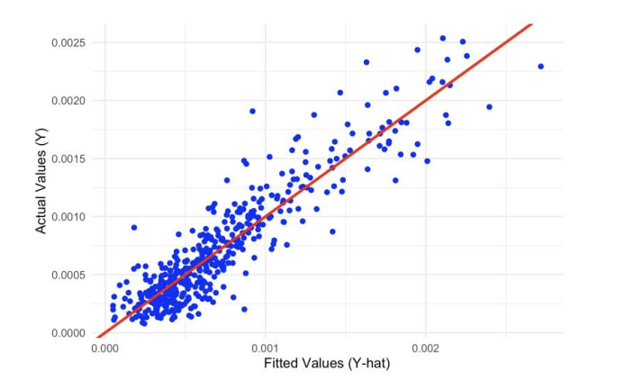
Model adequacy is evaluated against standard linear‑model conditions: linearity of the conditional mean, uncorrelated errors, homoskedastic disturbances, and approximately normal residuals. Plots of observed responses against fitted values show close alignment with the 45‑degree line, consistent with an adequate linear signal; deviations are small and unsystematic (Figure 5).

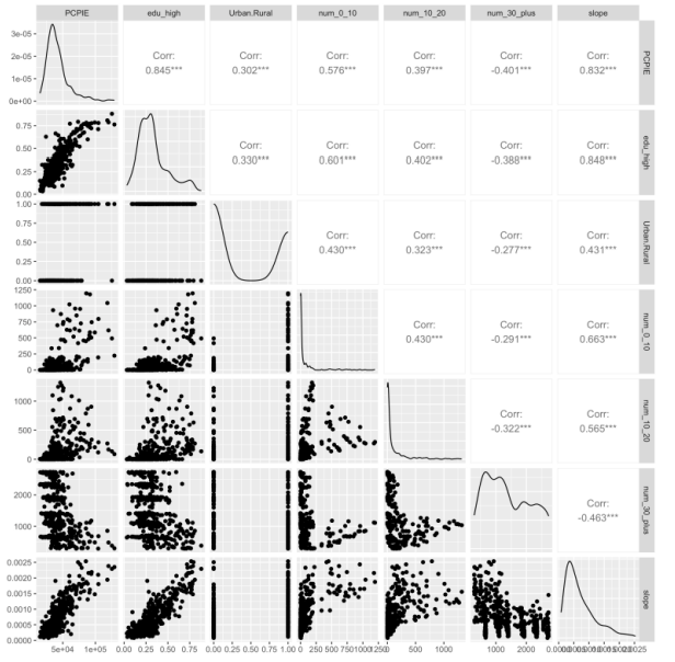
Pairwise associations among retained predictors appear roughly linear. Given the visual correlation between per‑capita income (PCPIE) and the high‑education share, we compute variance inflation factors (VIFs) to assess multicollinearity. All VIFs are below 5, indicating limited collinearity and no need to exclude additional predictors (Figure 6).

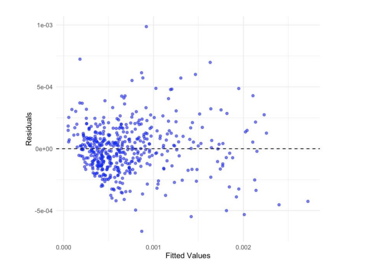
Residual‑versus‑fitted diagnostics show residuals centered near zero without pronounced curvature. A mild fan‑shape at higher fitted values suggests slight heteroskedasticity; to guard against size distortions in hypothesis tests, we report heteroskedasticity‑consistent (HC3) standard errors alongside conventional ones (Figure 7).

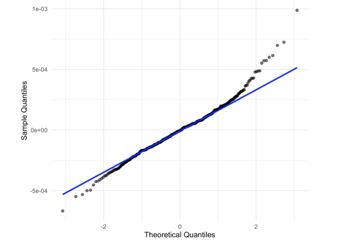
The normal Q–Q plot indicates residuals track the reference line closely with modest tail deviations, supporting approximate normality and the reliability of large‑sample inference (Figure 8).

Outliers, leverage points, and influential observations should be assessed to ensure model reliability. A data point is considered an outlier if its standardized residual lies outside the range of -4 to 4. A leverage point is one that is far from the mean of the predictor values and can substantially affect the fitted regression line. The threshold for leverage is defined as: 2 × (number of predictors + 1) / n,where n is the sample size.

Influential observations are identified using Cook’s Distance. A data point is considered influential if its Cook’s Distance exceeds the 50th percentile of the F distribution with degrees of freedom (p+1,n−p−1), where p is the number of predictors and n is the total number of observations.

By results, most standardized residuals fall within -4 and 4, with only a few potential outliers (e.g., observation 84). Cook’s Distance shows most points have low influence, with only a few exceeding the cutoff. Overall, the model is stable with limited influential cases.

4. Conclusion

This study quantifies ZIP-code–level EV adoption dynamics in Washington State over 2020–2025 by relating the monthly change in EV share to socioeconomic composition, urbanization, and the roll-out of public charging infrastructure. Multivariable linear models indicate that higher per-capita income, a larger share of highly educated residents, and urban status are each positively associated with faster growth in EV share. Access to charging infrastructure is salient at near distances: growth in the number of new stations within 0–10 miles and 10–20 miles is positively associated with adoption growth, whereas a greater concentration of distant stations (≥30 miles) is negatively associated with adoption, consistent with the distinct constraints of rural geographies. An interaction between urbanization and nearby station growth shows a weaker marginal association in urban ZIPs than in non-urban ZIPs, suggesting diminishing returns where baseline access is already high. These results answer the central questions posed in the Introduction by identifying the principal correlates of adoption and by demonstrating that spatial granularity at the ZIP level reveals localized patterns that broader geographies can obscure. Policy implications follow directly: charger siting decisions that prioritize proximity—particularly in underserved, lower-access areas—are likely to be more effective than strategies that expand distant infrastructure, and incentives targeted by local socioeconomic profiles may accelerate uptake where the marginal response is greatest. Overall, the findings provide an empirically grounded basis for fine-grained infrastructure planning and for designing geographically targeted incentives, while also motivating further causal analysis of infrastructure–adoption dynamics.

5. Discussion

Several considerations qualify the interpretation and indicate directions for further work. First, the outcome is a ZIP-level trend (the slope of monthly EV share), which improves comparability across places but does not by itself resolve endogeneity between charger deployment and demand. Infrastructure may be installed preferentially where adoption is already rising, potentially biasing naive associations upward. Future analyses should therefore incorporate identification strategies—such as panel fixed effects with time-varying controls, difference-in-differences around exogenous policy shocks, or instrumental variables exploiting program eligibility rules or grid siting constraints—to sharpen causal interpretation.

Second, the construction of the analytic dataset necessarily involved handling missing data and excluding manifest anomalies. Mean imputation for education shares was applied to fewer than ten percent of ZIPs to preserve coverage. This approach preserves coverage while acknowledging a potential attenuation of estimated effects, because mean imputation can shrink cross-sectional variance and bias coefficients toward zero; reporting heteroskedasticity- consistent standard errors (HC3) and comparing results to complete-case estimates partly mitigates concerns but does not eliminate them. Relatedly, exclusion thresholds—minimum cumulative registrations, extreme EV shares, implausible family sizes, and non-significant outcome trends—were set ex ante based on distributional evidence; sensitivity to alternative cutoffs is reported elsewhere and leaves the principal findings intact. Nonetheless, replication with alternative outlier rules and multiple-imputation procedures would further validate robustness.

Third, spatial structure may matter. Although fixed-radius counts of new stations offer transparent interpretation, spatial spillovers and network effects can induce dependence across neighboring ZIPs. Extensions using spatial error or spatial lag specifications, geographically weighted regression, or gravity-based accessibility indices could capture these interactions more explicitly. Likewise, aligning supply with potential demand via per-capita or per-vehicle accessibility, and distinguishing rapid-charging from lower-power stations, may refine effect heterogeneity. The documented weaker marginal association of nearby station growth in urban areas suggests diminishing returns in already dense networks; modeling nonlinearity (e.g., spline terms for charger access) would test this mechanism directly.

Finally, measurement and scope limitations remain. Registration and station inventories may contain dating or classification errors; charger operability and reliability are not observed; and important covariates—such as local electricity prices, parking availability, housing type, or model availability— are not yet integrated. Incorporating these factors, expanding beyond one state, and exploiting policy discontinuities would strengthen external validity and causal claims. Taken together, the present results underscore the importance of proximity-based infrastructure for accelerating adoption while highlighting methodological avenues—causal identification, richer spatial modeling, and improved data—to advance the evidence base.

Acknowledgement

Yiwen Xiong and Junqi Ling contributed equally to this work and should be considered co-first authors.

References

[1]. United States Environmental Protection Agency, “Transportation sector emissions | US EPA.” Mar. 2025, [Online]. Available: https: //www.epa.gov/ghgemissions/transportation-sector-emissions.
[2]. International Energy Agency, “Global EV outlook 2022, ” IEA, Paris, May 2022. [Online]. Available: https: //www.iea.org/reports/global-ev-outlook-2022.
[3]. M. Schulthoff, P. Anstett, J. Lange, D. Arend, E. Gencer, and M. Kaltschmitt, “Federal transformation costs of e-mobility in germany: Effectiveness and efficiency of EV incentives between 2015 and 2023, ” Transportation Research Interdisciplinary Perspectives, vol. 31, p. 101435, May 2025, doi: 10.1016/j.trip.2025.101435.
[4]. T. Lu, E. Yao, F. Jin, and Y. Yang, “Analysis of incentive policies for electric vehicle adoptions after the abolishment of purchase subsidy policy, ” Energy, vol. 239, p. 122136, 2022, doi: 10.1016/j.energy.2021.122136.
[5]. Z. He et al., “Examining the spatial mode in the early market for electric vehicles adoption: Evidence from 41 cities in china, ” Transportation Letters, vol. 14, no. 6, pp. 640–650, 2021, doi: 10.1080/19427867.2021.1917217.
[6]. D. L. Greene, E. Kontou, B. Borlaug, A. Brooker, and M. Muratori, “Public charging infrastructure for plug-in electric vehicles: What is it worth?” Transportation Research Part D: Transport and Environment, vol. 78, p. 102182, 2020, doi: 10.1016/j.trd.2019.11.011.
[7]. S. Ding and L. Wu, “Disparities in electric vehicle charging infrastructure distribution: A socio-spatial clustering study in king county, washington, ” Sustainable Cities and Society, vol. 121, p. 106193, Mar. 2025, doi: 10.1016/j.scs.2025.106193.
[8]. L. Luo, S. McLafferty, and F. Wang, “Analyzing spatial aggregation error in statistical models of late-stage cancer risk: A monte carlo simulation approach, ” International Journal of Health Geographics, vol. 9, p. 51, 2010, doi: 10.1186/1476-072X-9-51.
Cite this article
Xiong,Y.;Ling,J.;Wang,Y. (2025). ZIP-Code–Level Drivers of EV Adoption in Washington: Socioeconomics, Urbanization, and Charger Proximity (2020–2025). Applied and Computational Engineering,185,43-55.
Data availability
The datasets used and/or analyzed during the current study will be available from the authors upon reasonable request.
Disclaimer/Publisher's Note
The statements, opinions and data contained in all publications are solely those of the individual author(s) and contributor(s) and not of EWA Publishing and/or the editor(s). EWA Publishing and/or the editor(s) disclaim responsibility for any injury to people or property resulting from any ideas, methods, instructions or products referred to in the content.
About volume
Volume title: Proceedings of CONF-CDS 2025 Symposium: Application of Machine Learning in Engineering
© 2024 by the author(s). Licensee EWA Publishing, Oxford, UK. This article is an open access article distributed under the terms and
conditions of the Creative Commons Attribution (CC BY) license. Authors who
publish this series agree to the following terms:
1. Authors retain copyright and grant the series right of first publication with the work simultaneously licensed under a Creative Commons
Attribution License that allows others to share the work with an acknowledgment of the work's authorship and initial publication in this
series.
2. Authors are able to enter into separate, additional contractual arrangements for the non-exclusive distribution of the series's published
version of the work (e.g., post it to an institutional repository or publish it in a book), with an acknowledgment of its initial
publication in this series.
3. Authors are permitted and encouraged to post their work online (e.g., in institutional repositories or on their website) prior to and
during the submission process, as it can lead to productive exchanges, as well as earlier and greater citation of published work (See
Open access policy for details).