1.  Introduction

Weather forecasting plays an important role in daily life. It guides agricultural planning for planting and harvest. It helps transportation agencies prepare for severe weather and reduce risk. Energy providers can also optimize power and heating schedules [1]. Accurate forecasts create time windows for disaster prevention and loss reduction. Advances in observation have increased the volume and precision of data from satellites, radars, and sensors. These advances give data-driven methods a strong foundation [2]. Beyond traditional numerical weather prediction (NWP), many researchers now use machine learning and deep learning. These methods are flexible and adaptive. They can learn complex time patterns and nonlinear relations [3,4]. This study aims to predict short-term changes in air temperature and to compare three representative methods. A convolutional neural network (CNN) slides kernels along the time axis to extract local pattern changes. It captures short-term temperature fluctuations efficiently [5,6]. A Transformer uses self-attention to model dependencies over long sequences. It attends to global and local features at the same time. It suits meteorological data with long-range dependence [7-9].A random forest (RF) averages predictions from many decision trees. It offers robust performance, strong resistance to overfitting, and tolerance to outliers [10-12].By comparing these methods, we aim to reveal their strengths and limits for short-term temperature forecasting. The results can guide model choice and later optimization.

2.  Method

This study uses three representative methods to model and forecast short-term temperature. The methods are a Convolutional Neural Network (CNN), a Transformer model, and a Random Forest model. Each model has a distinct view of the data. Together, they help us understand and fit temperature patterns in time series.

2.1.  Convolutional Neural Network (CNN)

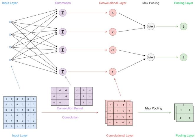
CNN is a deep neural network with local receptive fields and shared weights. Researchers use it widely in image and speech tasks.In time-series forecasting, a 1D convolution can extract local features from sequences. It captures short-term trends effectively [10,13].A CNN also uses fewer parameters than many traditional networks. It often trains faster and more stably [14]. We implement a 1D CNN in PyTorch. The input is the past 24 hours of temperature. The tensor shape is [batch_size,1,24]. The network stacks several convolution layers (nn.Conv1d). The activation is ReLU (nn.ReLU). Max-pooling layers (nn.MaxPool1d) reduce the feature length. A final fully connected layer (nn.Linear) outputs the predicted temperature for hour 25. We tune kernel size, channel count, and depth. The goal is to improve fit while keeping training stable.

1D convolution for a single input channel can be written as:

$$$ {\mathrm{y}}_{\mathrm{t}}=\sum _{\mathrm{i}=0}^{\mathrm{k}-1}{\mathrm{w}}_{\mathrm{i}}\bullet {\mathrm{x}}_{\mathrm{t}+\mathrm{i}}+\mathrm{b}$$$

 $$ \mathrm{x}$$ :the input sequence.

 $$ \mathrm{w}$$ :the convolution-kernel weights

 $$ \mathrm{b}:$$ the bias

 $$ \mathrm{k}$$ :the kernel size.

 $$ {\mathrm{y}}_{\mathrm{t}}$$ :the value of the output sequence at position t

The output of a convolution layer can be expressed formally as:

$$$ {{\mathrm{y}}_{\mathrm{t}}}^{\left(\mathrm{k}\right)}=\mathrm{\sigma }\bullet (\sum _{\mathrm{i}=0}^{\mathrm{K}-1}{{\mathrm{\omega }}_{\mathrm{t}}}^{\left(\mathrm{k}\right)}\bullet {\mathrm{x}}_{\mathrm{t}+\mathrm{i}}+{\mathrm{b}}^{\left(\mathrm{k}\right)})$$$

 $$ {{\mathrm{y}}_{\mathrm{t}}}^{\left(\mathrm{k}\right)}$$ :the output at position  $$ \mathrm{t}\mathrm{ }$$ from the  $$ {\mathrm{k}}^{\mathrm{t}\mathrm{h}}$$  kernel

 $$ {\mathrm{x}}_{\mathrm{t}+\mathrm{i}}$$ :is the  $$ {\mathrm{i}}^{\mathrm{t}\mathrm{ℎ}}$$  element of the input sequence starting at position  $$ \mathrm{t}$$ ;

 $$ {{\mathrm{\omega }}_{\mathrm{t}}}^{\left(\mathrm{k}\right)}$$ :is the  $$ {\mathrm{t}}^{\mathrm{t}\mathrm{ℎ}}$$  weight of the  $$ {\mathrm{k}}^{\mathrm{t}\mathrm{ℎ}}$$  kernel

 $$ {\mathrm{b}}^{\left(\mathrm{k}\right)}$$ :the bias of the  $$ {\mathrm{k}}^{\mathrm{t}\mathrm{ℎ}}$$  kernel

 $$ \mathrm{\sigma }$$ :a nonlinear activation function, such as ReLU

 $$ \mathrm{K}$$ :the kernel size

This formula shows the core computation in a CNN convolution layer. The layer applies a sliding window (the kernel) to the input sequence. It performs a weighted sum, adds a bias, and then uses an activation function to produce a feature value. Each kernel extracts a different local pattern, such as an upward trend or an abrupt change. Multiple kernels run in parallel and capture diverse features in the data. This design improves the model’s ability to sense complex fluctuations. In time-series tasks, this mechanism fits short-term dynamics especially well. It plays a key role in the final prediction.

2.2.  Transformer model

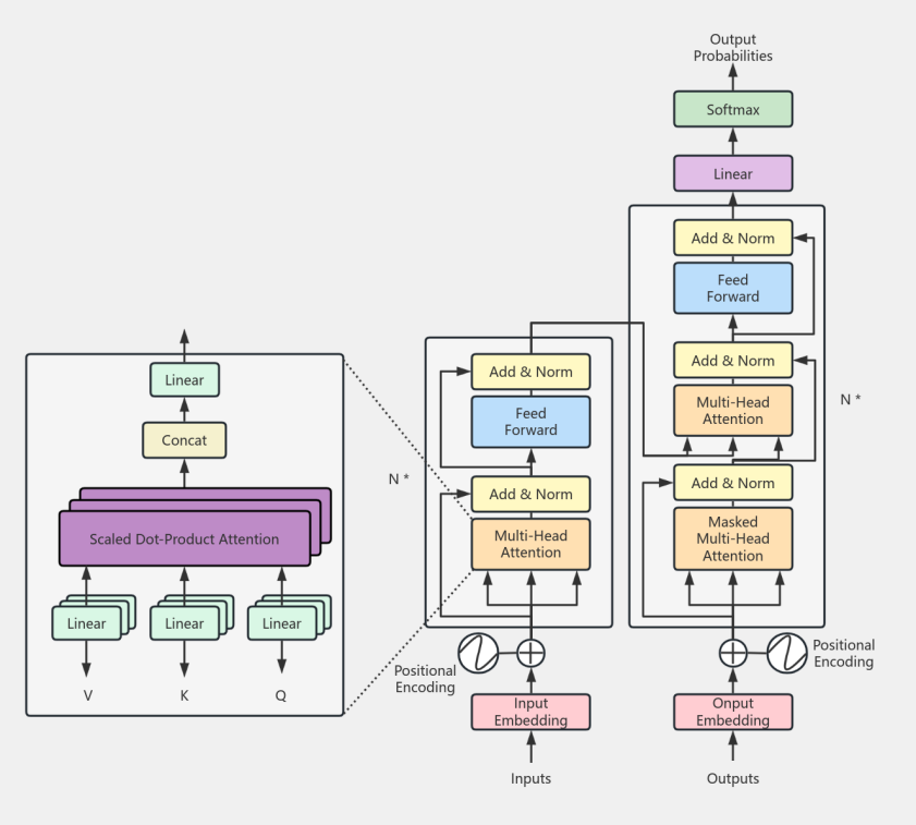
A Transformer is a neural network that relies only on attention. It was first used in natural language processing.Unlike an RNN, a Transformer does not pass information step by step in order.

The model uses self-attention to capture relations between all positions in the input.This design suits time series with long-range dependence.Its parallel computation also improves training efficiency [6,7].This study builds a simplified Transformer in PyTorch.The model uses two encoder layers (nn.TransformerEncoderLayer).Each layer contains multi-head self-attention and a feed-forward network.A linear embedding and a positional encoding first transform the temperature sequence. These steps let the model track time order [8]. The output is the predicted temperature at hour 25. We use the Adam optimizer and the mean squared error (MSE) loss.

Scaled Dot-Product Attention:

$$$ \mathrm{A}\mathrm{t}\mathrm{t}\mathrm{e}\mathrm{n}\mathrm{t}\mathrm{i}\mathrm{o}\mathrm{n}(\mathrm{Q},\mathrm{ }\mathrm{K},\mathrm{ }\mathrm{V})\mathrm{ }=\mathrm{ }\mathrm{s}\mathrm{o}\mathrm{f}\mathrm{t}\mathrm{m}\mathrm{a}\mathrm{x}\left(\frac{\mathrm{Q}{\mathrm{K}}^{\mathrm{T}}}{\sqrt{{\mathrm{d}}_{\mathrm{k}}}}\right)\mathrm{V}$$$

Here,  $$ \mathrm{Q}$$ ,  $$ \mathrm{K}$$ , and  $$ \mathrm{V}$$  are the query, key, and value vectors.The term  $$ {\mathrm{d}}_{\mathrm{k}}$$  is the key dimension.

Positional Encoding:

We use the standard sinusoidal positional encoding. The encoding adds order information to the embeddings.

$$$ {\mathrm{P}\mathrm{E}}_{(\mathrm{p}\mathrm{o}\mathrm{s},2\mathrm{i})}=\mathrm{s}\mathrm{i}\mathrm{n}\left(\frac{\mathrm{p}\mathrm{o}\mathrm{s}}{{10000}^{2\mathrm{i}/{\mathrm{d}}_{\mathrm{m}\mathrm{o}\mathrm{d}\mathrm{e}\mathrm{l}}}}\right),\mathrm{ }{\mathrm{P}\mathrm{E}}_{(\mathrm{p}\mathrm{o}\mathrm{s},2\mathrm{i}+1)}=\mathrm{c}\mathrm{o}\mathrm{s}\left(\frac{\mathrm{p}\mathrm{o}\mathrm{s}}{{10000}^{2\mathrm{i}/{\mathrm{d}}_{\mathrm{m}\mathrm{o}\mathrm{d}\mathrm{e}\mathrm{l}}}}\right)$$$

In addition to short-term prediction, Transformer-based architectures have been extended for long-horizon meteorological forecasting, demonstrating their effectiveness in capturing complex temporal dependencies [19].

2.3.  Random Forest (RF)

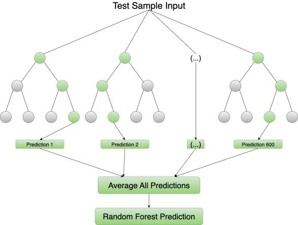
A Random Forest is an ensemble learning method. The model builds many decision trees and combines their outputs. The approach improves accuracy and stability [13].The method is non-parametric and resists overfitting. It often works well when data are limited or structure is simple.

We use RandomForestRegressor from scikit-learn. The input is the past 24 hours of temperature. The target is the temperature at hour 25. Key parameters include n_estimators = 100 and an auto-selected max_depth. The model does not require feature scaling. The model also does not rely on time order. The method suits tasks with clear feature structure.

For regression, the forest averages tree outputs:

$$$ \widehat{\mathrm{y}}=\frac{1}{\mathrm{N}}\sum _{\mathrm{i}=1}^{\mathrm{N}}{\mathrm{T}}_{\mathrm{i}}\left(\mathrm{x}\right)$$$

 $$ {\mathrm{T}}_{\mathrm{i}}\left(\mathrm{x}\right)$$  : the prediction from the $$ {\mathrm{ }\mathrm{i}}^{\mathrm{t}\mathrm{ℎ}}$$  tree. $$ \mathrm{N}$$  : the total number of trees. $$ \widehat{\mathrm{y}}$$  : the final prediction.

3.  Result

3.1.  Experimental data

We use the Beijing PM2.5 dataset from the UCI repository. The dataset records hourly weather from 2010 to 2014 for one area in Beijing. The variables include PM2.5, temperature, humidity, pressure, wind speed, and precipitation. In this experiment, we set temperature as the target. The goal is to predict a future temperature from recent observations.

We preprocess the data in Python. We use pandas and numpy for cleaning and normalization. We apply Z-score normalization to each variable. We then build supervised samples with a sliding window. The input is 24 consecutive hours of temperature. The target is the temperature at hour 25. We split the data in time order into a training set (70%) and a test set (30%). The test set is not used during training.

3.2.  Experimental setup

All models take the same input. The input is the past 24 hours of temperature. The output is the temperature at hour 25. We use the same train and test splits for all models to ensure fairness.

The CNN uses 1-D convolution. We tune the number of channels and the kernel size.The Transformer uses two encoder layers. Each layer has multi-head attention and a feed-forward network.The Random Forest tests several parameter groups. We vary the number of trees, the maximum depth, and the minimum samples per leaf. We search for a good configuration.

We run the experiments on Windows 11 Pro. The machine has an AMD Ryzen 9 7945HX CPU, 32 GB RAM, and a discrete GPU with 16 GB VRAM. The setup supports stable and efficient training and testing.We compare three models: CNN, Transformer, and Random Forest. The target variable is temperature from the Beijing PM2.5 dataset. All models use the same input format. We input the past 24 hours and predict hour 25. We tune hyperparameters for each model. We then evaluate test-set prediction accuracy to compare fit and generalization under different settings.

This table shows the effect of learning rate on CNN performance under a fixed architecture. The model fits best when the learning rate is between 0.0020 and 0.0026. The test  $$ {\mathrm{R}}^2$$  values cluster around 0.930. This range balances convergence speed and error reduction. The CNN shows strong local feature extraction. The model captures short-term temperature swings effectively.

The Transformer is more sensitive to the learning rate. The best result appears at a learning rate of 0.0016, with an  $$ {\mathrm{R}}^2$$  of 0.9266. The model relies on long-range dependence and shows smooth trends with smaller error swings [8]. However, the response to extreme values is slower. This lag can make short-term forecasts slightly weaker than those of the CNN.

This table reports RF performance under different parameter sets. The results show small gains as the number of trees increases, but the overall change is minor. The  $$ {\mathrm{R}}^2$$  values stay stable between 0.930 and 0.932, which indicates strong robustness and generalization. The best  $$ {\mathrm{R}}^2$$  is 0.9319 at n_estimators = 200, min_samples_leaf = 3, and max_depth = 20. On this dataset, added complexity brings only marginal returns. The strength of the forest comes mainly from the ensemble, not from deeper single trees.

The CNN performs best at learning rates from 0.0023 to 0.0026, with  $$ {\mathrm{R}}^2$$ ≥0.930. The model suits short-term fluctuation capture. The Transformer is more sensitive to the learning rate and peaks at 0.0016 with $$ {\mathrm{R}}^2$$ =0.9266. The model suits global trend capture. The Random Forest is stable across settings and reaches a top  $$ {\mathrm{R}}^2$$  of 0.9319. Its predictions look slightly less smooth, but training is fast and noise resistance is strong.

Deep models are slightly more accurate than the traditional model, but they are less efficient than the Random Forest in training complexity and resource use [8]. Different models shine in different settings. Deep learning offers higher accuracy but demands more tuning and compute. Future work can try ensembling, add more weather variables, and include external signals such as pollution sources and human activity. These steps may improve practical value and accuracy.

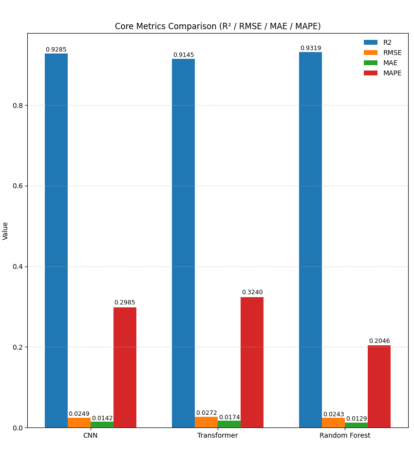
Error metrics support these points. The Random Forest shows clear advantages in RMSE, MAE, and MAPE. Its MAPE is lower than that of the CNN and the Transformer, which shows stronger robustness to outliers and extreme swings [14,15]. Explained variance results show that RF and CNN have similar feature-explanation ability, and both exceed the Transformer [16]. Inference latency also matters. The CNN and RF can respond in milliseconds. The Transformer is slower, but it has potential for long-range dependence [17]. For short-term temperature prediction, RF is an efficient and stable baseline. The CNN can add extra accuracy when the dataset is larger.

This figure compares the three models on core metrics for temperature forecasting. The metrics are  $$ {\mathrm{R}}^2$$ , RMSE, MAE, and MAPE.

Random Forest reaches the highest  $$ {\mathrm{R}}^2$$  at 0.9319. The model shows the best overall predictive power. CNN follows with  $$ {\mathrm{R}}^2$$  = 0.9285. The model has an edge in capturing short-term local patterns. Transformer scores lower at  $$ {\mathrm{R}}^2$$= 0.9145. The gap likely reflects limits from data scale and structural complexity [18,19].

We also observe clear error advantages for Random Forest. The model has the lowest MAE and MAPE. The result indicates strong stability and robustness to outliers. Recent research also suggests that ensemble deep learning can further improve robustness by mitigating single-model bias [20]. CNN delivers accuracy close to Random Forest and remains competitive Compared with these two models, the Transformer has a theoretical strength for long-range dependence. However, the model does not perform as well with small samples.

Overall, Random Forest shows high accuracy and strong stability on this dataset. CNN achieves near-RF accuracy. The two approaches suggest that classical machine learning and deep learning can complement each other in practical forecasting.

4.  Conclusion

In the actual application of meteorological prediction, the model selection should be balanced with the task characteristics and resource conditions: for the scenarios requiring rapid deployment, limited data scale or limited computing resources, the traditional machine learning method still has practical value; While in the pursuit of higher prediction accuracy and the use of rich historical data and computing resources, the deep learning model can provide better performance. In addition, the integration of multiple models, the introduction of more meteorological and external factors, or the combination of physical models and data-driven methods have the potential to further improve the accuracy and stability of short-term temperature prediction.

References

[1]. J. Ahn, J. Kim, and Y. Park, "Deep learning approaches for weather forecasting: A review, " Atmosphere, vol. 15, no. 1, p. 123, 2024. doi: 10.3390/atmos15010123.
[2]. C. Wen, Z. Fu, Y. Guo, and Q. Zhou, "Deep learning for weather and climate prediction: A survey, " Artif. Intell. Rev., vol. 55, no. 8, pp. 5977–6006, 2022. doi: 10.1007/s10462-021-10083-1.
[3]. P. Hewage, A. Behera, M. Trovati, and E. Pereira, "Machine learning approaches for weather and climate modelling, " Neurocomputing, vol. 461, pp. 237–256, 2021. doi: 10.1016/j.neucom.2021.07.045.
[4]. M. Reichstein, G. Camps-Valls, B. Stevens, M. Jung, J. Denzler, N. Carvalhais, and P. Prabhat, "Deep learning and process understanding for data-driven Earth system science, " Nature, vol. 566, no. 7743, pp. 195–204, 2019. doi: 10.1038/s41586-019-0912-1.
[5]. A. Krizhevsky, I. Sutskever, and G. E. Hinton, "ImageNet classification with deep convolutional neural networks, " Adv. Neural Inf. Process. Syst., vol. 25, pp. 1097–1105, 2012.
[6]. K. He, X. Zhang, S. Ren, and J. Sun, "Deep residual learning for image recognition, " Proc. IEEE Conf. Comput. Vis. Pattern Recognit. (CVPR), pp. 770–778, 2016. doi: 10.1109/CVPR.2016.90.
[7]. A. Vaswani et al., "Attention is all you need, " Adv. Neural Inf. Process. Syst., vol. 30, pp. 5998–6008, 2017.
[8]. H. Zhou, S. Zhang, J. Peng, S. Zhang, J. Li, H. Xiong, and W. Zhang, "Informer: Beyond efficient transformer for long sequence time-series forecasting, " Proc. AAAI Conf. Artif. Intell., vol. 35, no. 12, pp. 11106–11115, 2023.
[9]. L. Breiman, "Random forests, " Machine Learn., vol. 45, no. 1, pp. 5–32, 2001. doi: 10.1023/A: 1010933404324.
[10]. X. Li and Y. Qian, "CNN-based approaches for short-term weather prediction, " J. Appl. Meteorol. Climatol., vol. 63, no. 2, pp. 245–260, 2024.
[11]. Y. Li, H. Zhang, and J. Wang, "Application of random forests in meteorological forecasting, " Theor. Appl. Climatol., vol. 157, no. 3–4, pp. 789–803, 2024.
[12]. J. A. Weyn, D. R. Durran, and R. Caruana, "Can machines learn to predict weather? Using deep learning to predict gridded 500-hPa geopotential height from historical weather data, " J. Adv. Modeling Earth Syst., vol. 11, no. 8, pp. 2680–2693, 2019. doi: 10.1029/2019MS001705.
[13]. S. Wang, Y. Liu, X. Chen, and J. Zhu, "Hybrid models for weather prediction combining deep learning and physical approaches, " Clim. Dyn., vol. 60, no. 1–2, pp. 55–70, 2023. doi: 10.1007/s00382-022-06410-7.
[14]. J. Chen, L. Zhao, and Y. Huang, "Evaluation of error metrics in weather forecasting models, " Environ. Model. Softw., vol. 162, p. 105589, 2023. doi: 10.1016/j.envsoft.2023.105589.
[15]. R. J. Hyndman and A. B. Koehler, "Another look at measures of forecast accuracy, " Int. J. Forecasting, vol. 22, no. 4, pp. 679–688, 2006. doi: 10.1016/j.ijforecast.2006.03.001.
[16]. R. Lam, Q. He, and T. Zhang, "Explainable AI in weather forecasting: Current progress and future directions, " Expert Syst. Appl., vol. 213, p. 118957, 2023. doi: 10.1016/j.eswa.2022.118957.
[17]. P. D. Dueben and P. Bauer, "Challenges and design choices for global weather and climate models based on machine learning, " Geosci. Model Dev., vol. 11, no. 10, pp. 3999–4009, 2018. doi: 10.5194/gmd-11-3999-2018.
[18]. S. Rasp, P. D. Dueben, S. Scher, J. A. Weyn, S. Mouatadid, and N. Thuerey, "WeatherBench: A benchmark dataset for data-driven weather forecasting, " J. Adv. Modeling Earth Syst., vol. 12, no. 11, e2020MS002203, 2020. doi: 10.1029/2020MS002203.
[19]. K. Bi, Z. Sun, and X. Zhao, "Robust weather forecasting models using ensemble deep learning, " Appl. Intell., vol. 53, no. 5, pp. 5431–5445, 2023. doi: 10.1007/s10489-022-04077-8.
[20]. Y. Liu, T. Xu, X. Chen, and W. Zhang, "Transformer-based models for weather forecasting: A comprehensive study, " IEEE Trans. Geosci. Remote Sens., vol. 60, pp. 1–15, 2022. doi: 10.1109/TGRS.2021.3137264.
Cite this article
Feng,Q. (2025). A Comparative Study on Deep Learning-Based: Temperature Prediction Models: Performance Evaluation of CNN, Transformer and Random Forest. Applied and Computational Engineering,191,1-10.
Data availability
The datasets used and/or analyzed during the current study will be available from the authors upon reasonable request.
Disclaimer/Publisher's Note
The statements, opinions and data contained in all publications are solely those of the individual author(s) and contributor(s) and not of EWA Publishing and/or the editor(s). EWA Publishing and/or the editor(s) disclaim responsibility for any injury to people or property resulting from any ideas, methods, instructions or products referred to in the content.
About volume
Volume title: Proceedings of CONF-MLA 2025 Symposium: Intelligent Systems and Automation: AI Models, IoT, and Robotic Algorithms
© 2024 by the author(s). Licensee EWA Publishing, Oxford, UK. This article is an open access article distributed under the terms and
conditions of the Creative Commons Attribution (CC BY) license. Authors who
publish this series agree to the following terms:
1. Authors retain copyright and grant the series right of first publication with the work simultaneously licensed under a Creative Commons
Attribution License that allows others to share the work with an acknowledgment of the work's authorship and initial publication in this
series.
2. Authors are able to enter into separate, additional contractual arrangements for the non-exclusive distribution of the series's published
version of the work (e.g., post it to an institutional repository or publish it in a book), with an acknowledgment of its initial
publication in this series.
3. Authors are permitted and encouraged to post their work online (e.g., in institutional repositories or on their website) prior to and
during the submission process, as it can lead to productive exchanges, as well as earlier and greater citation of published work (See
Open access policy for details).