1. Introduction

Automatic technology, which offers tremendous convenience while reducing labor costs, has increasingly gained popularity in people's work and daily lives as a result of the continuous development of relevant technologies. Path planning, a way of finding a collision-free route from the initial position to the destination using a set of assessment criteria, is one of the key autonomous driving technologies. Global and local path planning are two types of path planning [1]. The process of choosing the best way from one place to another across an environment, taking into account all barriers and other limitations, is known as global path planning. Robotics, driverless cars, and computer graphics are several of the industries that use it. The A*, Dijkstra, Rapidly-Exploring Random Trees (RRT), Genetic, and Ant Colony Optimization methods are examples of global path planning algorithms [2,3]. These algorithms offer great search capabilities, but are computationally difficult and inefficient. Local path planning provides a mobile robot with a trajectory that is feasible and safe to navigate in a given environment, based on its current state and perception of the environment. This trajectory is typically planned over a short distance, and its goal is to avoid obstacles and reach a desired destination while satisfying various constraints such as collision avoidance, minimum turning radius, and maximum velocity. Fuzzy Logic, Artificial Potential Field (APF), Reinforcement Learning, and Simulated Annealing (SA) methods are mostly used for local path planning [4].

Oussama Khatib raised the APF in 1986 [5,6]. It is a method of obtaining a predetermined path by driving the robot's motion through an artificially designed potential field, which has become one of the classical algorithms in robot navigation. At present, APF method has been widely used and studied in robot navigation, autonomous control, target tracking and other fields. The implementation of APF is simple, with fast computation and a wide range of applications. But at the same time, there are problems such as local minima, influenced by initial parameters, unsmooth paths, etc. Many efforts have been made to amend the APF. Li et al. looked at algorithms already used for robot path planning and focused on using APF when there are static barriers and unknown environmental factors [7]; for second-order multi-agent formation, Qin et al. studied the APF-based impulsive consensus problem, where the control technique is provided and validated [8]; Sun et al. investigated the local optimum problem of conventional APF approach and introduced the obstacle function of gravity to solve the defects that the UAV falls into local optimum and the target unreachability [9]; He et al. suggested and tested an improved algorithm based on SA for the problems like local minima of conventional APF [10].

In order to overcome the local minima of the conventional APF approach and provide a fair route to the target location, a modified algorithm is provided in this study.

2. Traditional artificial potential field

The idea of this algorithm is to convert a path planning problem into a robot motion problem due to forces in the environment. The robot is made to avoid impediments in its way and eventually arrive at the target spot by creating a virtual potential field in the area.

In the environment, an obstacle will generate a repulsive field around it, while the target point will generate a global attractive field. The repulsive field decreases as the distance to the obstacle increases and when the distance is beyond a specific range, the repulsive field is zero. In other words, when the distance is too far, the obstacle will not have any impact on the robot. It makes sense to consider the impact radius of obstacles as the safe distance between the robot and an obstacle. The repulsive field takes the following form as shown in formula (1).

\( {U_{rep}}(x)=\begin{cases} \begin{array}{c} \frac{1}{2}k(\frac{1}{l(x,{x_{0}})}-\frac{1}{{x_{0}}}), 0≤l(x,{x_{0}})≤{x_{0}} \\ 0 , l(x,{x_{0}}) \gt {x_{0}} \end{array} \end{cases} \) (1)

In the equation, \( k \) is a constant proportional to the repulsive field, \( x \) is the position of the robot, \( {x_{0}} \) is the position of the obstacle, and \( l(x,{x_{0}}) \) is the distance in between. There’s a limit of the distance \( l(x,{x_{0}}) \) marked as \( {x_{0}} \) . Only when the distance is smaller than this value \( {x_{0}} \) , does repulsive field exist. If a robot gets into the safe distance of an obstacle (into the repulsive potential field), the obstacle will exert repulsive force on it. The associated field's negative gradient represents the repulsive force, as shown in formula (2).

\( \vec{{F_{rep}}}(x)=\begin{cases} \begin{array}{c} \frac{1}{2}k(\frac{1}{l(x,{x_{0}})}-\frac{1}{{x_{0}}})\frac{1}{{l^{2}}(x,{x_{0}})}∇ x(x,{x_{0}}), 0≤l(x,{x_{0}})≤{x_{0}} \\ 0 , l(x,{x_{0}}) \gt {x_{0}} \end{array} \end{cases} \) (2)

The attractive field has a universal range, and as the robot moves away from the target point, the attractive force acting on it grows. The attractive force becomes less powerful as the robot approaches the desired location, and once it reaches the target spot, it no longer affects the robot.

The expression of the repulsive field is shown in formula (3), where \( {x_{g}} \) is the position of the destination, \( l(x,{x_{g}}) \) is the distance between the robot and its goal, \( ε \) is the proportional gain of the field. The corresponding attractive field force is shown in formula (4).

\( {U_{att}}(x)=\frac{1}{2}ε{l(x,{x_{g}})^{2}} \) (3)

\( \vec{{F_{att}}}(x)=-∇{U_{att}}(x)=εl(x,{x_{g}}) \) (4)

Combining the two types of forces results in the total force acting on the robot, and formula (5) illustrates this statement.

\( \vec{{F_{tol}}}(x)=\vec{{F_{att}}}(x)+\sum _{i=1}^{m}\vec{{F_{rep}}}(x) \) (5)

Suppose there are m obstacles that will exert repulsive forces on the robot. The cumulative force acting on the robot determines its mobility, and figure 1 depicts the robot's strength performance.

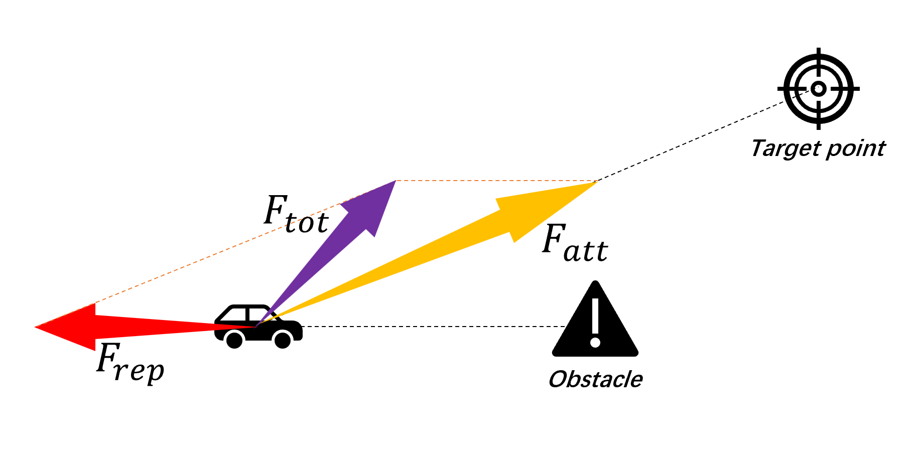
Figure 1. Robot forces analysis.

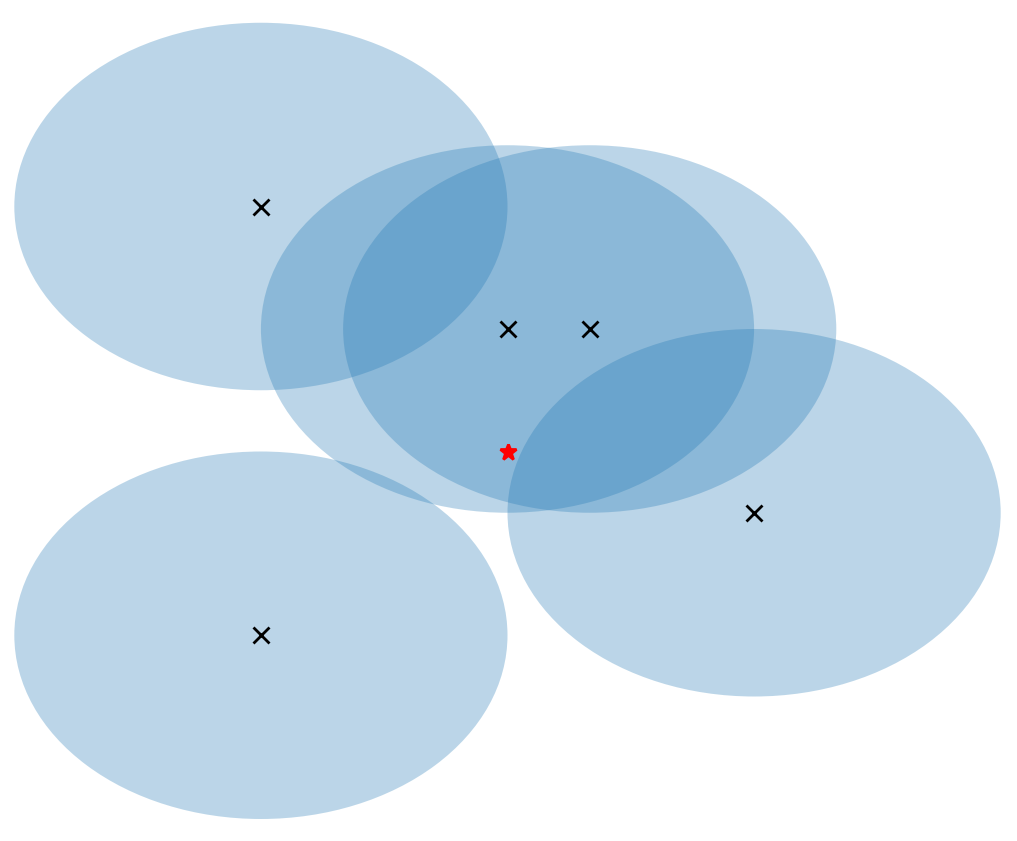
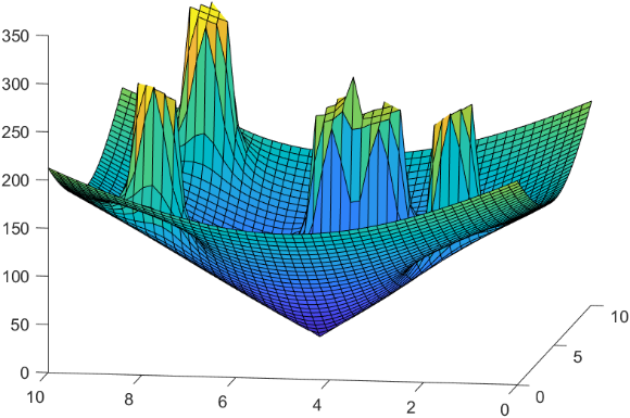
Figure 2 displays the target and obstacle distribution as well as the corresponding 3-dimensional potential field map. In the picture, X represents the obstacle, the blue circles around X indicates its repulsive influence range (safe distance), and the red star represents the target point. Figure 2 (a) shows the distribution of obstacles and target points, and figure 2 (b) shows their corresponding 3D potential field map. As can be seen, if all the field energy is converted into potential energy, the obstacles are the hills in the environment and the target points are the valleys. When puting a ball (the robot) into the environment, it will automatically travel to the valley (target) point, bypassing those hills (obstacles) in the process.

3. Improved artificial potential field

Since the conventional APF only takes into account local information around the robot, the robot may encounter some local minimum points before reaching the target point. The robot will stop at some local optimum point or oscillate in a very small range, thus not reaching the target point. To solve this problem, this paper utilizes odometry to determine whether the robot is trapped in a local minimum and makes the robot move in a direction perpendicular to the repulsive force with increasing steps to get rid of this local minima. The following is the flowchart of this algorithm in figure 3.

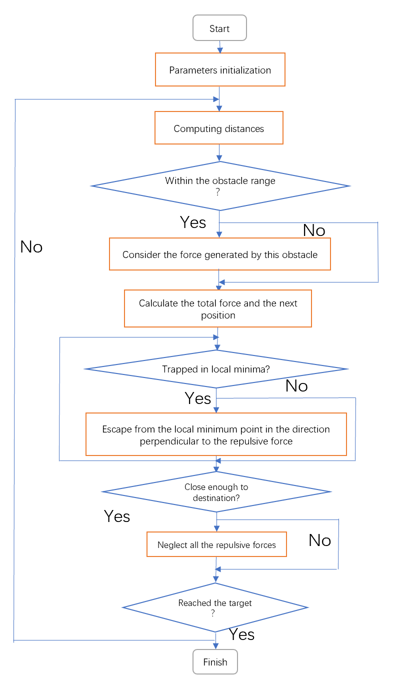
Figure 3. Workflow of the improved APF.

3.1. Judgment on falling into local minima

Intuitively, a robot stuck at a local minimum point is depicted as remaining in one spot or constantly jittering about a certain center. All that needs to be done is determine the largest distance between the robot's location coordinates during a certain amount of time. With the use of this data, whether the robot has reached a local minimum is determined. If this maximum distance is less than a suitably tiny constant ρ, it is safe to believe that the robot has entered a local minimum.

When it comes to 'a certain period of time', it’s alright to take it as a certain number of steps. In this algorithm, the maximum distance \( ρ \) , between the last tens of positions of the robot (e.g., take the last 30 steps) is observed for the determination of the robot being trapped in a local minimum. If \( ρ≤δ \) ,then the robot is determined to have fallen into the local minima.

The value of the threshold \( δ \) is extremely crucial, and the magnitude of this threshold should be determined by actual circumstances. If \( δ \) is taken too small, it will be too difficult to detect the local minimum, and if the value of \( δ \) is too large, many locations that are not local minimums may be mistaken for local minimums, and the robot will frequently take escape measures, which is more wasteful of energy. Simulations proved that the threshold \( δ \) should be taken at 1 to 2 times the step size \( θ \) . Generally, it is best to take it 1.5 times, that is, \( δ=1.5θ. \)

3.2. Escape from local minima

After the robot is captured at a local minima, it's about time to plan an escape. The robot is made to move in increasing steps in the direction perpendicular to the repulsive force until it escapes from the local minimum. After the robot reaches a local minimum point, this algorithm's technique is used, and the robot can then leap out of this local minimum and advance along a trajectory that resembles an obstacle contour.

The escape step length, for example, can start from twice the set step length, and gradually increase into multiples (3 times, 4 times, 5 times...).

3.3. Solution for target unreachable in the final stage

If there are obstacles very close to the desired point (the target point is even within the area of influence of the obstacles), the combined action of the repulsive field and the attractive field will produce local minima at some locations around the target. Thus, the robot will be very likely to fall into these local minimum points. Although it is already close enough to the target point, the motion state is balanced here due to the local optimum, so it will not make it to the desired position. As a result, in this algorithm, when the robot is close enough to the target point, it will ignore all the effects of repulsive forces. The robot is then allowed to reach its destination successfully under the influence of the attractive force when its distance to the destination is less than a threshold \( γ \) . Obviously, obstacle avoidance is prioritized when the target point is far away, and arrival is prioritized when the destination is near.

The value of threshold \( γ \) is also of great significance. If \( γ \) is taken too small, even less than the distance from the local minima points discussed above to the goal, this correction method will not work at all and the robot will still be trapped there; if \( γ \) is taken too large, it will be too early for the robot to eliminate the influence of all repulsive forces, which may contribute to collisions with obstacles and thus cannot successfully implement obstacle avoidance. \( γ \) should not be taken larger than the impact radius (safety distance \( {p_{0}} \) ) of the obstacle repulsive force. Simulations have shown that it is generally appropriate to take \( γ={p_{0}}/3 \) .

4. Simulation results

The feasibility, correctness and robustness of this algorithm were verified by simulations carried out with Pycharm software, and the simulation results of conventional APF and this modified APF were recorded for comparison. Figure 4 to figure 6 show the results generated by conventional and improved algorithms under the case of local minima, where X represents obstacles, the blue circles around X indicates the repulsive influence range (safe distance), the red triangle represents the initial position, the red star represents the goal position, and the blue dots indicate the robot’s trajectory. In this simulation, the robot is treated as a mass point.

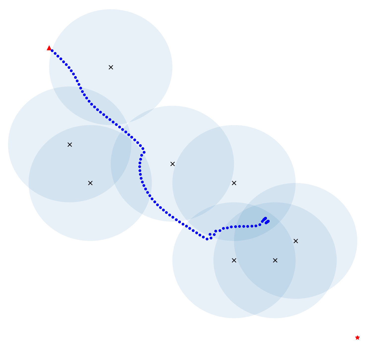
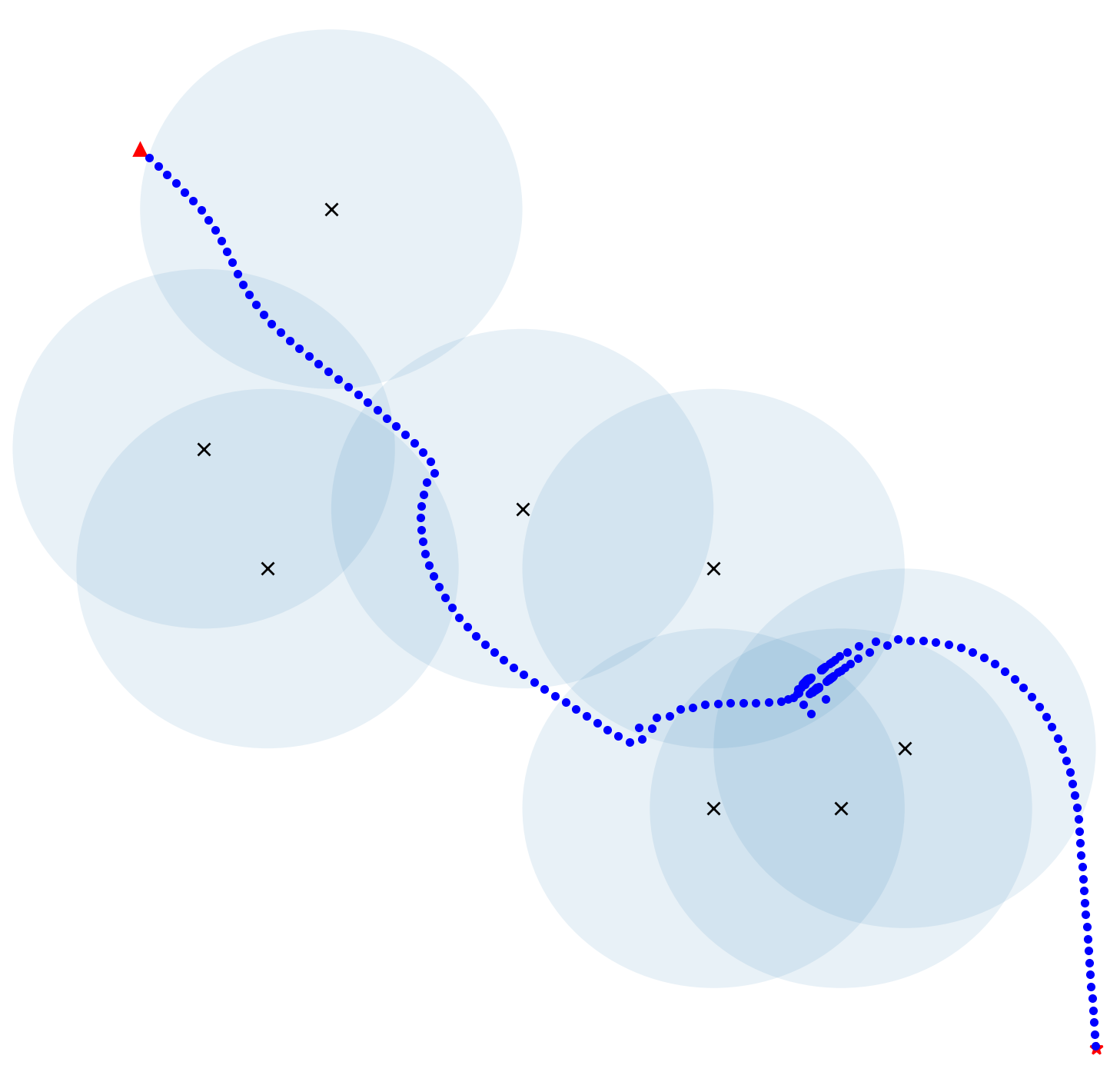
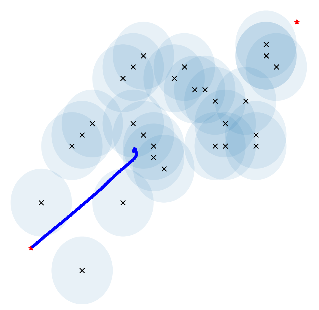
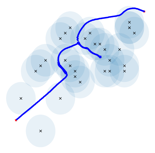
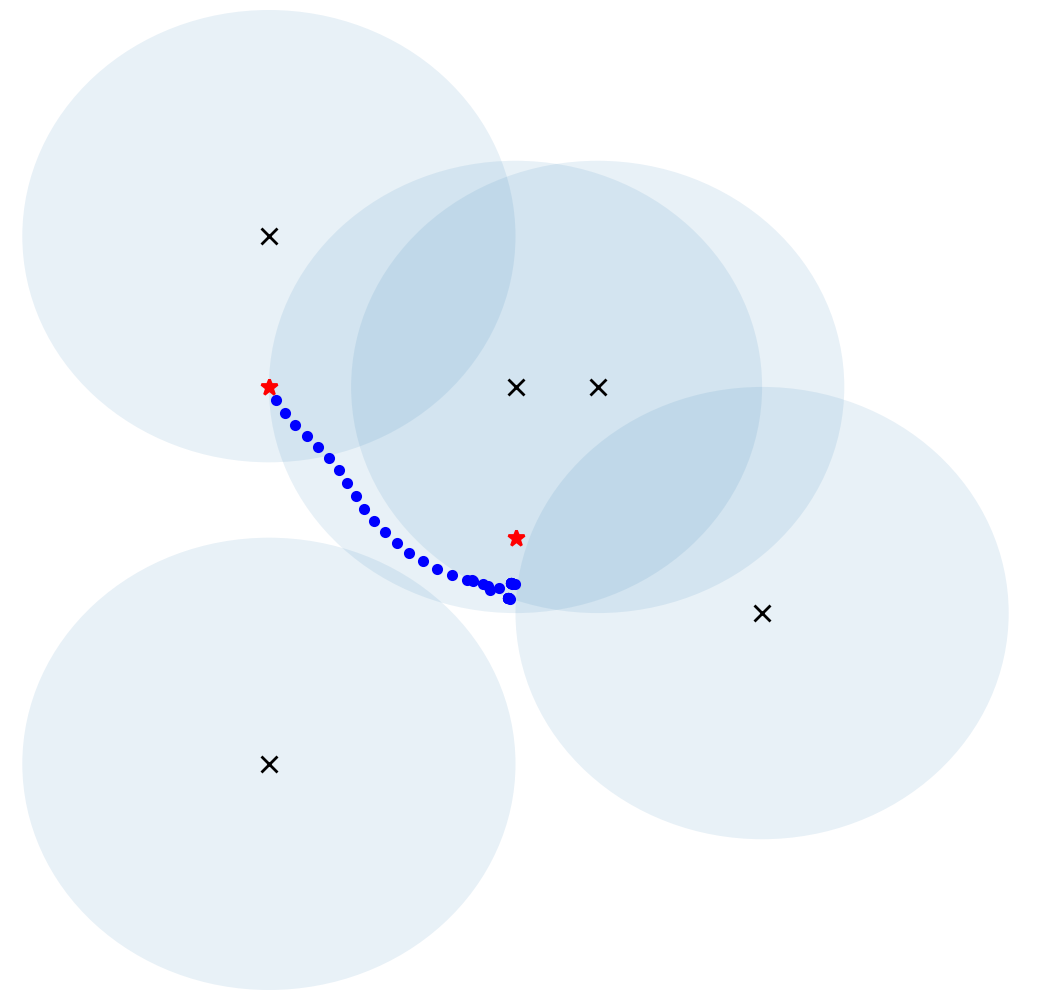
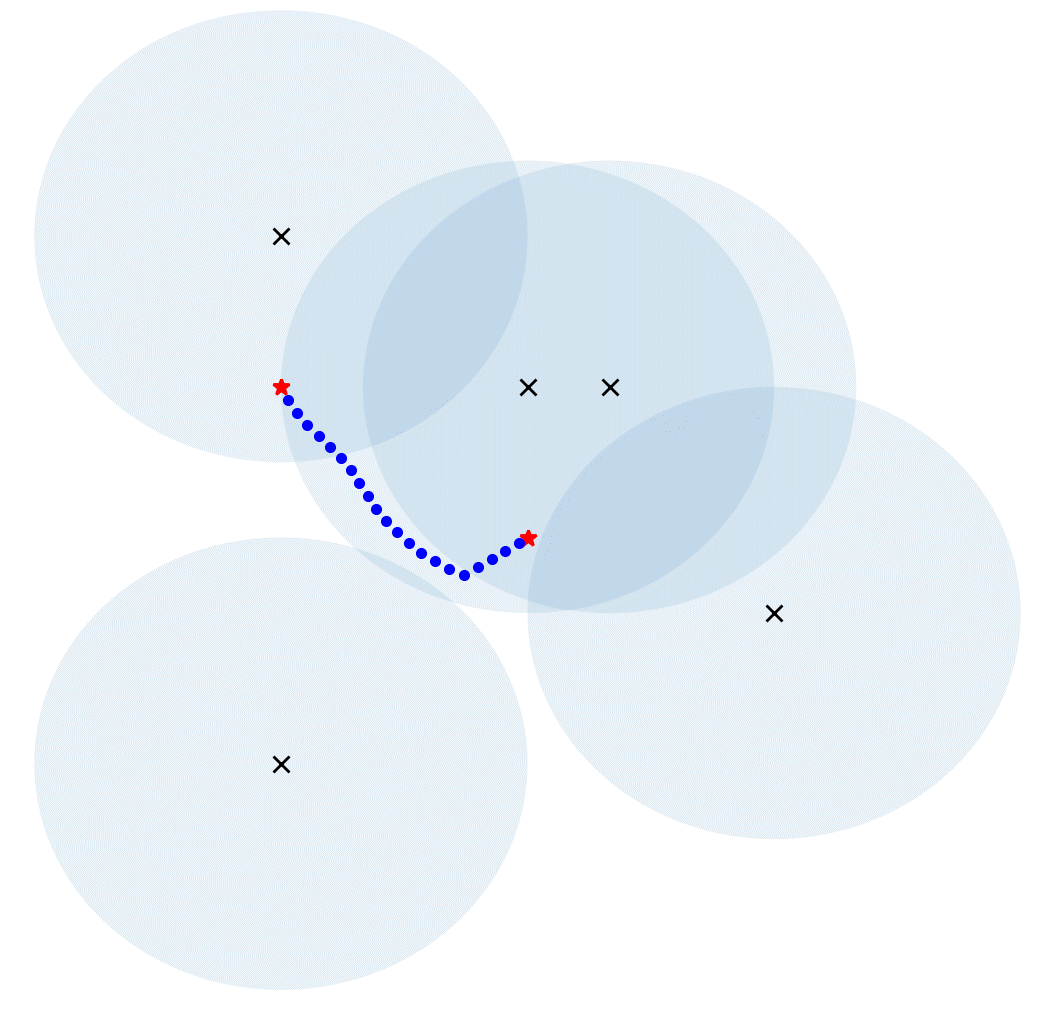
Compared with conventional APF, the method in this paper can effectively have the problems of local minima solved. As illustrated in the figures above, this algorithm can save the robot from the local minima, bypass barriers, and get to the goal point in the end. Whenever a robot falls into a new local minimum point, it could escape in the same way. Moreover, the algorithm proved to be robust because it works well in various situations.

Figure 4 shows a relatively simple and common situation, which can be easily solved by applying this algorithm. Figure 5 shows a very complex situation where there are many obstacles and the robot is separated from its destination by several walls. Applying this algorithm also let the robot to reach the destination in a reasonable trajectory without collisions. However, it should be noted that the robot's trajectory is broken in figure 5(b), which means that the robot took a rather big step there. This will cause the robot to travel unsteadily and have some impact on the machine. Furthermore, it can be noticed that the robot in figure 5 has an extremely twisting and roundabout track. The robot kept trying and making mistakes, which would lead to a waste of energy. In the case shown in figure 6 (a), although the robot almost reached the target point, it just couldn’t accomplish an arrival due to the presence of obstacles near the destination, which create repulsive forces on the robot. In this algorithm, when the robot gets close enough to its goal, this issue may be solved by disregarding the repelling impact of any barriers. In the final stage, the robot is pulled to the goal by the target point.

5. Conclusion

A modified APF approach is proposed in this study. It includes identifying the local minima by odometry, escaping the local minimum point by increasing the step size in the direction perpendicular to the repulsive force until it escapes successfully, and finally ignoring the repulsive field influence when close enough to the target. Simulations illustrate that this approach is feasible and effective in solving the local minima, and it is robust in different situations.

However, on the one hand, the automatic tracing process of this algorithm can be random and circuitous, which could result in a waste of energy and time. On the other hand, gradually increasing the escape step length will make the robot action unstable and have some certain impact on the robot. In response to these existing problems, further study is expected to be taken, such as integrating A* Algorithm or DQN Algorithm, managing to smoothen the path and robot’s action and so on.

The future trends of artificial potential fields are varied and unpredictable, including integration with Machine Learning, works on Swarm Robotics, Hybrid Approaches, application in Human-Robot Collaboration and so on. However, the potential for APF algorithms to revolutionize the way people work with robotics is high, and it can be expected to see an increasing adoption of this technology in the coming years.

References

[1]. Z. Liangbo, Z. Guangsheng, Z. Ling and J. Pinghui 2021 Improved Research on Target Unreachable Problem of Path Planning Based on Artificial Potential Field for an Unmanned Aerial Vehicle, 2021 IEEE 7th International Conference on Control Science and Systems Engineering (ICCSSE), Qingdao, China pp. 136-142.
[2]. L. Tian and C. Collins 2014 An effective AGV trajectory planning method using a genetic algorithm, Mechatronics, Vol.14, pp.455-470.
[3]. A. Ammar, H. Bennaceur, I. Châari, A. Koubâa, and M. Alajlan 2015 Relaxed Dijkstra and A* with linear complexity for AGV path planning problems in large-scale grid environments, Soft Computing, Vol. 20, pp. 4149-4174.A. Ammar, H. Bennaceur, I. Châari, A. Koubâa, and M. Alajlan 2015 Relaxed Dijkstra and A* with linear complexity for AGV path planning problems in large-scale grid environments, Soft Computing, Vol. 20, pp. 4149-4174.A. Ammar, H. Bennaceur, I. Châari, A. Koubâa, and M. Alajlan 2015 Relaxed Dijkstra and A* with linear complexity for AGV path planning problems in large-scale grid environments, Soft Computing, Vol. 20, pp. 4149-4174.
[4]. C. Zheyi and X. Bing 2021 AGV Path Planning Based on Improved Artificial Potential Field Method, 2021 IEEE International Conference on Power Electronics, Computer Applications (ICPECA), Shenyang, China pp. 32-37.
[5]. O. Khatib 1986 Real-Time Obstacle Avoidance for Manipulators and Mobile Robots, International Journal of Robotics Research, vol. 5, pp. 90-98.
[6]. O. Khatib 1986 The Potential Field Approach and Operational Space Formulation in Robot Control. Springer, New York.
[7]. Li, B. Tian, Y. Yang and C. Li 2022 Path planning of robot based on artificial potential field method, 2022 IEEE 6th Information Technology and Mechatronics Engineering Conference (ITOEC), Chongqing, China pp. 91-94.
[8]. Y. Qin, Z. Liu, L. Fu, Z. Dong, Q. Sun and D. He 2021 Impulsive Consensus Algorithms for Second-order Multi-agent Formation Based on the Improved Artificial Potential Field, 2021 International Conference on Neuromorphic Computing(ICNC), Wuhan, China, pp.188-193.
[9]. Y. Sun, W. Chen and J. Lv 2022 Uav Path Planning Based on Improved Artificial Potential Field Method, 2022 International Conference on Computer Network, Electronic and Automation (ICCNEA), Xi'an, China, pp. 95-100.
[10]. He, Y. Su, j. Guo, X. Fan, Z. Liu and B. Wang 2020 Dynamic path planning of mobile robot based on artificial potential field, 2020 International Conference on Intelligent Computing and Human-Computer Interaction (ICHCI), Sanya, China, pp. 259-264.
Cite this article
Miao,F. (2023). Improved artificial potential field method for local minima. Applied and Computational Engineering,10,47-54.
Data availability
The datasets used and/or analyzed during the current study will be available from the authors upon reasonable request.
Disclaimer/Publisher's Note
The statements, opinions and data contained in all publications are solely those of the individual author(s) and contributor(s) and not of EWA Publishing and/or the editor(s). EWA Publishing and/or the editor(s) disclaim responsibility for any injury to people or property resulting from any ideas, methods, instructions or products referred to in the content.
About volume
Volume title: Proceedings of the 2023 International Conference on Mechatronics and Smart Systems
© 2024 by the author(s). Licensee EWA Publishing, Oxford, UK. This article is an open access article distributed under the terms and
conditions of the Creative Commons Attribution (CC BY) license. Authors who
publish this series agree to the following terms:
1. Authors retain copyright and grant the series right of first publication with the work simultaneously licensed under a Creative Commons
Attribution License that allows others to share the work with an acknowledgment of the work's authorship and initial publication in this
series.
2. Authors are able to enter into separate, additional contractual arrangements for the non-exclusive distribution of the series's published
version of the work (e.g., post it to an institutional repository or publish it in a book), with an acknowledgment of its initial
publication in this series.
3. Authors are permitted and encouraged to post their work online (e.g., in institutional repositories or on their website) prior to and
during the submission process, as it can lead to productive exchanges, as well as earlier and greater citation of published work (See
Open access policy for details).