


1. Introduction
Although numerous researchers have conducted extensive research on financial market forecasting, few studies have compared the efficacy of machine learning (i.e., ML) and deep learning (i.e., DL) techniques in stock market forecasting problem. This paper compares and analyses the effectiveness of DL and traditional ML in stock market forecasting. The novelty of this paper is the introduction of data visualization techniques for preprocessing the data prior to modelling to assist in selecting the most appropriate model. Various metrics are used to contrast model prediction results and assess their performance. This paper demonstrates the significance of data visualization in stock market forecasting based on these operations.
As a result of the current economy's reliance on financial investments, investors are continuously searching for more accurate methods to predict market performance. Today, global financial markets assume an essential part in the growth of a globalized economy, and the stock market ranks among the most frequently discussed areas regarding various financial investments [1, 2]. In the past, investors predicted the financial sector using traditional technical and fundamental evaluation methods. Fundamental analysis consists of assessing the investment value of a stock by analyzing fundamental indicators such as a company's financial statements, operating performance, and industry outlook. Technical analysis, on the other hand, involves analyzing a stock's historical price action, trading volume, volatility and other technical indicators to predict a stock's future price action. These methods have limitations since the market's nature constantly changes and evolves [3].
The primary focus of this paper is an overview of stock market forecasting and a comparison of the application and performance assessment of traditional ML and DL forecasting techniques. Deep convolutional neural networks (i.e., CNN) [4] can significantly enhance the accuracy of stock market forecasting and assist investors in making better investment decisions, as determined by comparing various models. The paper then discusses the advantages of data visualization for comprehending market behavior and trends, such as providing insight into stock price patterns and trends, detecting correlations between various stocks, and facilitating decision-making.
This paper examines the following topics: What are the advantages and disadvantages of utilizing traditional ML techniques to foresee the stock exchange? Can DL techniques enhance the precision of stock market forecasts? What are the benefits of utilizing data visualization for stock market forecasting?
2. Literature surveys
Predictions of stock price movements are generated using CNN and long short-term memory networks (i.e., LSTM) [5]. Other conventional ML techniques, such as logistic regression (i.e., LR), support vector machines (i.e., SVM), and decision trees, were compared to CNN and LSTM models. The results suggest that methods employing CNN and LSTM can produce superior prediction performance with a 10% decrease in mean absolute error (MAE) compared to conventional methods.
According to Mehtab et al. [6], DL-based convolutional neural networks (CNNs) were more effective than traditional methods in predicting stock market movements. Their research demonstrated that DL techniques could capture nonlinear data relationships and increase prediction accuracy.
Better predictions of stock market movements were made using ML-based techniques. Studies showed that ML methods were more suitable for handling large-scale and high-dimensional data, thus improving the stability and accuracy of forecasts [7]. The findings suggested that artificial intelligence techniques, especially DL, had a promising future in various fields.
Utilizing visualization technologies have also benefited stock market analysis. Saeed et al. [8] analyzed the impact of the COVID-19 outbreak on the Pakistan Stock Exchange's stock returns and volatility. Their data visualization demonstrated that the pandemic significantly affected the market, with various sectors exhibiting varying returns. According to Hoseinzade [9], numerous stock market variables were utilized to increase the accuracy of predictions. The final research findings show that the CNN model predicts the stock market with high accuracy and robustness and can utilize diverse data to improve prediction accuracy.
This paper examines the stock market trend forecasting research using artificial intelligence and data visualization techniques as the primary instruments. The techniques employed are LR, SVM, multi-layer perceptron (i.e., MLP) and CNN. Some studies test the epidemic's impact on the financial markets. Such studies demonstrate that artificial intelligence and data visualization techniques can enhance the understanding and prediction of stock market movements, the accuracy and stability of forecasts, and decision support for policymakers and businesses.
3. Introduction of algorithms
3.1. Machine learning techniques
3.1.1. Logistic regression. Logistic regression (i.e., LR) [10] applies to dichotomous and multiclass classification problems. Training efficiency and model interpretation are among their strong points. In the stock market, LR can be used to predict the increase or decrease of stock values and determine the optimal moment to buy or sell stocks. LR is a prevalent classification algorithm based on linear regression. A sigmoid function maps the output of linear regression. This output generates a probability value ranging from 0 to 1, indicating the likelihood that a sample falls into a specific category. If this probability surpasses 0.5, the sample is classed as belonging to this category. For probabilities less than 0.5, reverse the order of the probabilities.
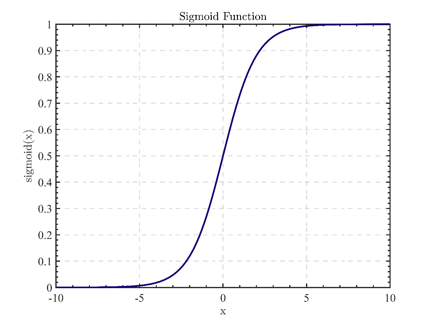
Figure 1. The sigmoid function.
The sigmoid function may be expressed as an activation function for logistic regression, specifically as equation (1):
| (1) |

where e refers to the base of natural logarithms, in figure 1, and x is a linear combination that converges to 0 or 1 by substituting huge positive or small negative numbers into the sigmoid function.
Accuracy, precision, recall, and F1 score are frequently utilized metrics in LR. These metrics can be used to assess the efficacy and precision of a model during model selection and optimization.
Typically, the data sources include historical stock prices, volume, trading hours, and additional information. This information is accessible via financial websites, exchanges, and other channels.
3.1.2. Support vector machine. SVM [11] is a supervised learning approach for classification and regression problems. SVM aims to identify the optimal hyperplane for separating diverse data classes. The hyperplane is an n-1 dimensional linear classifier, where n refers to the number of parameters. The margin, or distance from the classification boundary, allows SVM to classify data.
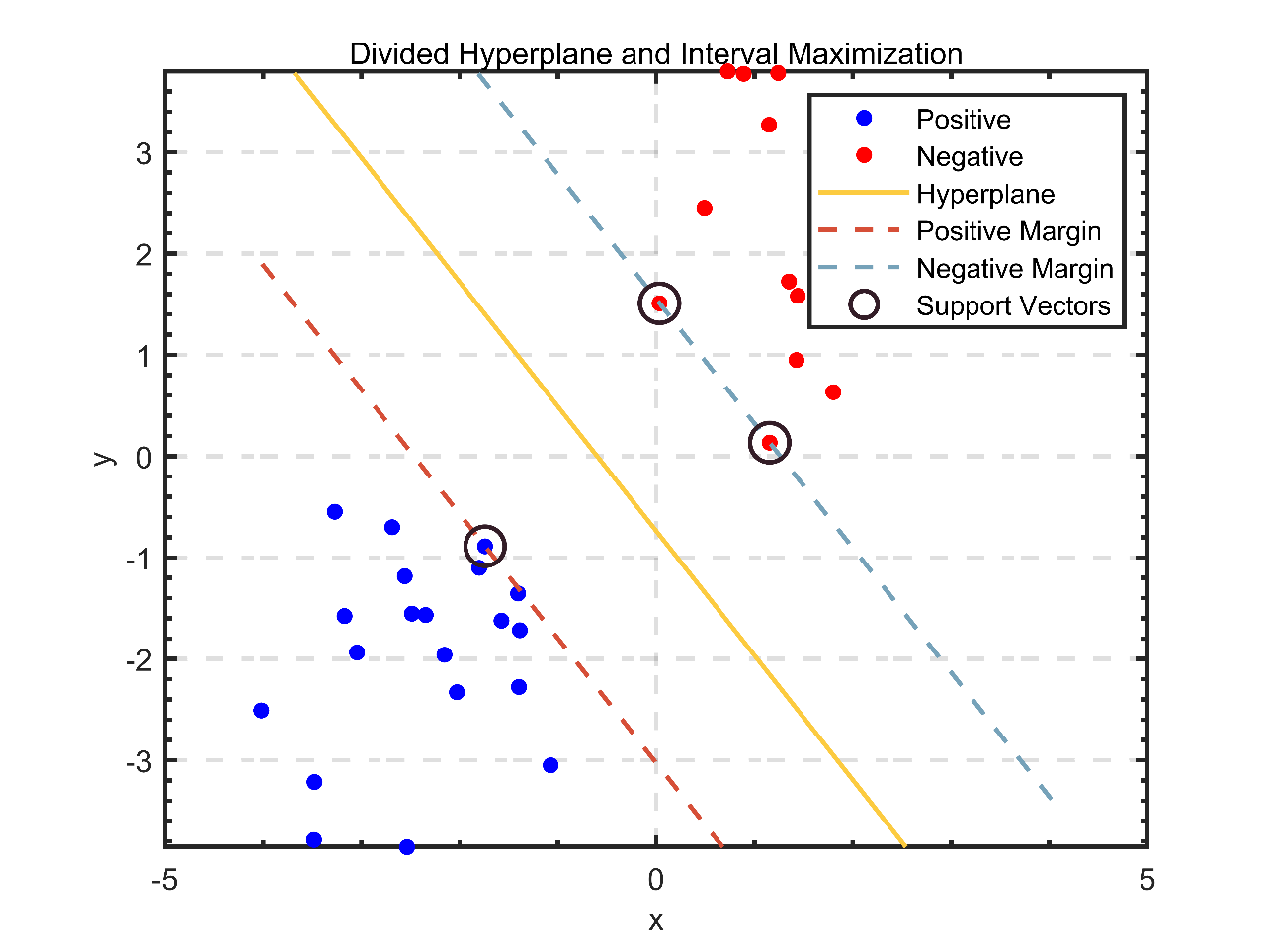
Figure 2. Divided hyperplane and interval maximization.
Both data points on the sides of any hyperplane have a minimum distance from it, the sum of which is the margin. In figure 2, the black line depicts the optimal hyperplane that divides the data into two categories. The red and blue dashed lines represent the hyperplane's boundaries, also known as the decision boundary. The points on the dashed lines represent the support vectors, the locations closest to the decision boundary. The SVM will identify a hyperplane for segmentation that can distinguish between the two classes and maximize the margin. A superior segmentation hyperplane has the most negligible effect on local perturbations of the sample, generates the most robust classification results, and generalizes most effectively to unobserved examples.
In SVM, classification accuracy and interval size are the most critical metrics. Classification accuracy measures the proportion of correct classifications the model makes on the test data set. The interval size quantifies the distance between the classification boundary and the training sample closest to the boundary. A larger interval is generally indicative of improved generalization performance.
Text, images, and numeric data can serve as the data source for SVM. SVM requires the data features are pre-processed, which typically entails two steps: feature extraction and feature selection. Extraction of features transforms the original data into a feature representation that the model can use. Feature selection is selecting the most relevant extracted features to enhance the generalization ability and precision of a model's predictions.
3.2. Deep learning techniques
3.2.1. Multi-layer perceptron. Multiple layers of neurons are present in Multi-layer Perceptron (i.e., MLP) [12], a variety of artificial neural networks. MLP is a feedforward neural network, which suggests that information flows unidirectionally from input to output layers. Similar to other neural networks, MLPs are employed to recognize patterns in unprocessed data and to aid in the resolution of complex problems.
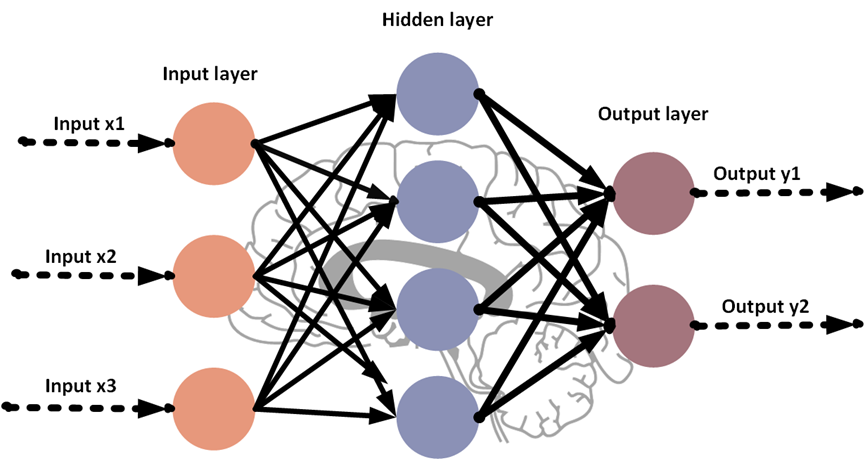
Figure3. The infrastructure of MLP.
In figure 3, the three inputs are sent from the input neurons to the first hidden neurons, which also contain multiple neurons. Each of hidden neurons receives all three inputs and computes a weight value. An activation function transforms these weighted aggregates to generate the output of the first hidden layer. The output of the first concealed layer is the input for the subsequent concealed layer. Similarly, each node in the following hidden layer calculates the weight value of its inputs and modifies them by utilizing the activation function to produce the output of that layer. This process is repeated four times until the last concealed stratum is reached. Each neuron in both output layers evaluates a weighted sum of its inputs, which an activation function transforms to generate an output. MLPs are applicable for classification, regression, and clustering tasks. They frequently use performance metrics, including accuracy, precision, recall, F1 value, etc.
In stock market forecasting, MLPs are often used to predict stock prices and trends to help investors make decisions. MLPs require enough historical data as input to learn stock price patterns and trends, and they need to process and downscale the data appropriately, such as normalization, feature selection, and dimensionality reduction, to avoid overfitting. Also, MLPs can be continuously improved based on the new inputs obtained.
3.2.2. Convolutional neural network. CNN [13] is a methodology for DL that is also primarily used for image recognition, target detection, and speech recognition, among other applications.
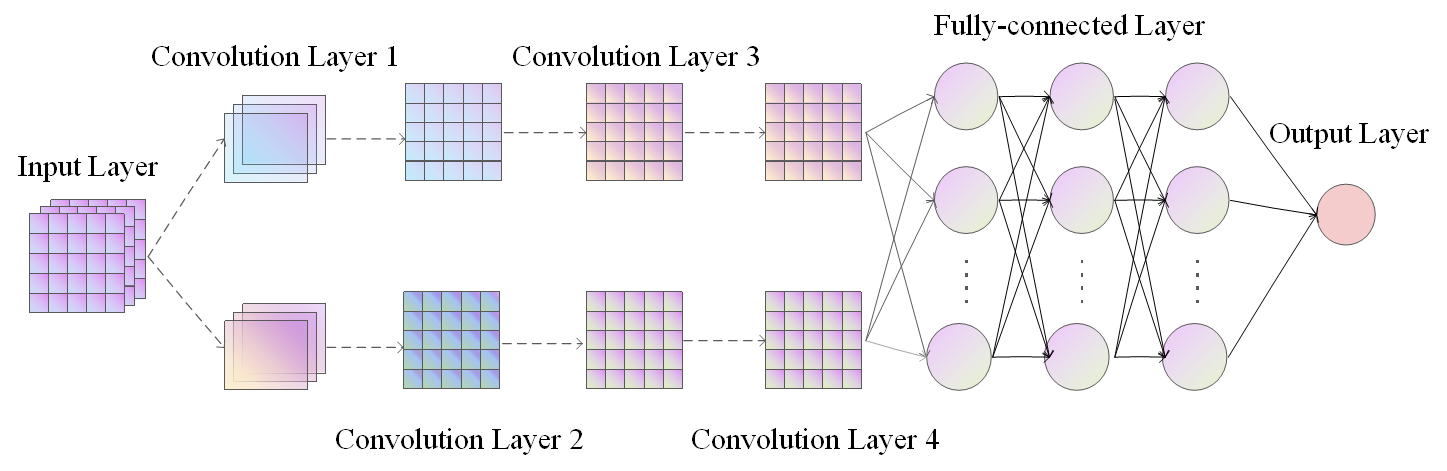
Figure 4. The framework of CNN.
Figure 4 illustrates the architecture of a CNN model. This network consists of four convolutional layers and three completely interconnected layers.
In this architecture, the first convolution layer has sixteen 3x3-sized filters and generates 64 feature maps. Each filter in the 2nd convolution operation is 3x3, and the layer generates 32 feature maps. Every filter in the 3rd convolution operation has a 3x3 dimension, and the layer generates sixteen feature maps. Each of the 128 3x3 filters in the 4th convolution operation generates eight feature maps. These feature maps are transmitted to the output layer via the fully-connected layer, which then classifies its images following the feature map values. This structure consists of three entirely connected layers, with the first and second layers containing 128 neurons and the third layer containing ten neurons.
In stock market prediction, CNNs are often used to analyze charts and technical indicators of stock prices. CNNs can take as input price change data and technical indicators, and then extract features through convolutional and pooling layers. These traits can assist CNN in comprehending the patterns and regularities of price fluctuations. Last but not least, the fully-connected layer can predict future stock prices by correlating image patches with output.
4. A comparison of LR, SVM and MLP algorithms
On a small dataset, this work contrasts the stock market forecasting performance of three algorithms: LR, SVM and MLP.
In this paper, the S&P 500 dataset is pre-processed by normalizing the data to assure their stability and reliability. The previous five days' closing price, opening price, and trading volume were chosen as inputs for feature selection.
The SVM model uses the radial foundation function as the kernel function and modifies its penalty and kernel coefficients. The LR model uses the Logistic Regression class from the scikit-learn library. The MLP model consists of a neural network with two hidden layers, the relu activation function and the Adam optimizer.
After training and testing, the performance of the LR, SVM and MLP models was evaluated on the S&P 500 dataset. Table 1 shows the results:
Table 1. Model comparison.
Model | Accuracy | F1 value | Top-1 error rate |
LR | 52.74% | 0.53 | 47.26% |
SVM | 54.45% | 0.54 | 45.55% |
MLP | 57.12% | 0.56 | 42.88% |
Based on the data presented in table 1, bar graphs are created to compare the three models.
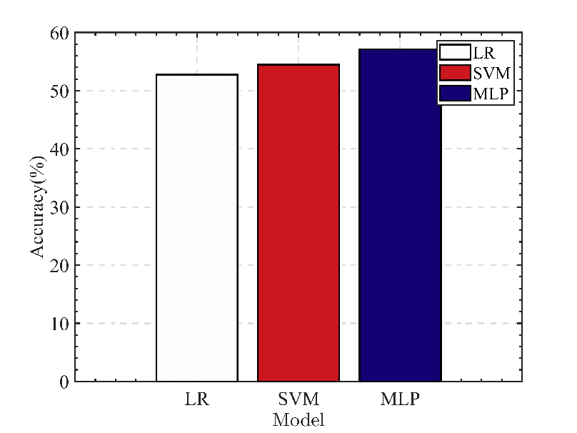
Figure 5. Comparison of accuracy.
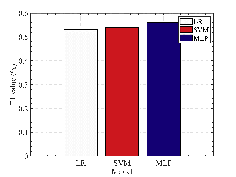
Figure 6. Comparison of F1 value.
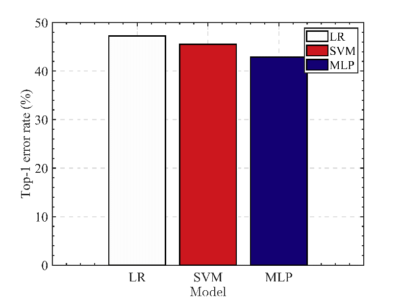
Figure 7. Comparison of Top-1 error rate.
Based on the above experimental results and the visualization method of bar graphs (see figure 5-7), it can be concluded that MLP performs the best among the three algorithms for predicting the stock market. Regarding prediction accuracy, F1 value, and Top-1 error rate, the MLP model on the S&P 500 data set outperformed the LR and SVM models. In particular, the test set accuracy of the MLP model was 57%, its F1 value was 0.56, and its Top-1 error rate was 43%. In contrast, the LR model has an accuracy of 52.74% on the test set, an F1 value of 0.53 and a Top-1 error rate of 47.26%, while the SVM model has an accuracy of 54.45% on the test set, an F1 value of 0.54 as well as a Top-1 error rate of 45.55%. These comparisons demonstrate that the MLP algorithm outperforms the LR and SVM algorithms regarding S&P 500 prediction results. The result may be due to the MLP algorithm's ability to capture nonlinear data relationships and its enhanced ability to learn complex patterns, resulting in improved stock market prediction performance.
In conclusion, based on the experimental results, the MLP algorithm outperforms the other two regarding stock market prediction.
4.1. Challenges
By comparing these algorithms, the following issues may be identified.
4.1.1. The problem of low accuracy. As demonstrated by the test results, the accuracy of all three models ranges between 50% and 60 %. One possible reason is that the stock market is highly complex and uncertain, making it difficult to make accurate predictions using simple models. Using more complex models or combining multiple models for integrated learning to enhance the forecasting performance of the models could be a potential solution to this issue.
In their paper, Broomhead et al. [14] compare the outcomes of integrating three models with individual models. It was demonstrated that the integrated learning models outperformed the individual models in terms of prediction performance, as well as accuracy, recall, and F1 values.
4.1.2. Uncertainty in model selection. Although the performance of the three models is comparable, different models apply to different data and tasks. Choosing the appropriate model is an important issue. The solution to this problem is to select the most suitable model by cross-validation and parameter tuning and to monitor and update the model in real time in real applications.
To this end, a regularized cross-validation method is proposed to reduce the estimated variance of generalization errors by limiting the number of overlapping samples, thus enabling efficient algorithm comparisons [15]. In addition, the paper extends the regularized cross-validation method to textual datasets and gives a corresponding Bayesian test.
5. CNN's application to the market for stocks
Hyun et al. [16] created a CNN and technical analysis-based asset prices forecasting model in order to assess the viability of the innovative learning method in the share market. They employed the CNN model to create images of time series graphs using a variety of technical indicators used in technical analysis as input variables for the prediction model. This study contrasts the prediction accuracy of the proposed model to that of the MLP model and the SVM model to validate DL's capacity for stock market image recognition.
The data used in this analysis span from 10:30 p.m. on April 3, 2017, to 12:15 p.m. on May 2, 2017. The duration of the entire data compilation is 41,250 seconds. The time ratio between the training data set and the test data set is 4:1. Every 30 minutes, time series data were converted to images, with 1100 images used for training and 275 for assessment.
The MLP model uses a sigmoid activation function, three hidden layers, and one remote unit. For its nonlinear classification, the SVM employs a polynomial kernel.
They compiled a group of technical indicators for the prediction model. They also employed a strike rate, sensitivity, and specificity index to determine the model's predictive accuracy.
| (2) |
| (3) |
| (4) |


where n0,0 and n0,1 measure the frequency with which 1 was anticipated while the actual value was 0, and vice versa. For the number of times 0 was predicted when the actual value was 0.
Four CNN models with distinct technical metric inputs were developed. In this investigation, these models were also designated CNN1, CNN2, CNN3, and CNN4. Table 2 lists the input variables for these four models, as presented in [16].
Table 2. The variables used by CNN model.
Model Number | Input variables |
CNN1 | Closing price |
CNN2 | Closing price, SMA, EMA |
CNN3 | Closing price, SMA, EMA, ROC, MACD |
CNN4 | Closing Price, SMA, EMA, ROC, MACD, Fast %K, Slow %D, Upper Band, Lower Band |
Similarly, the variants of MLP and SVM are also denoted by MLP1, MLP2, MLP3, MLP4, SVM1, SVM2, SVM3 and SVM4. The obtained information of the accuracy scores for the three models, including MLP, SVM, CNN and their variants, are reported in table 3. It is worthy noting that numbers are originally reported by [16].
Table 3. The accuracy scores of MLP, SVM and CNN models.
Model | Hit ratio | Specificity | Sensitivity |
MLP1 | 0.4872 | 0.6866 | 0.2979 |
SVM1 | 0.48 | 0.8881 | 0.0922 |
CNN1 | 0.85 | 0.9593 | 0.6971 |
MLP2 | 0.5602 | 0.5674 | 0.5522 |
SVM2 | 0.4655 | 0.8582 | 0.0922 |
CNN2 | 0.62 | 0.6679 | 0.5878 |
MLP3 | 0.5653 | 0.6561 | 0.4801 |
SVM3 | 0.5018 | 0.4851 | 0.5177 |
CNN3 | 0.64 | 0.9559 | 0.2487 |
SVM4 | 0.5455 | 0.5149 | 0.5745 |
MLP4 | 0.5573 | 0.6269 | 0.4626 |
CNN4 | 0.66 | 0.6548 | 0.6872 |
The CNN models have the most excellent hit rate compared to all other models in table 3. Additionally, its specificity and sensitivity are higher than other models, which indicates that the CNN model has superior true-negative and true-positive rates and can more accurately distinguish positive and negative cases.
In conclusion, the prediction performance of MLP and SVM is inferior to that of CNN; therefore, using CNN with input images can be an effective method for predicting financial markets.
5.1. Challenges
The results of this experiment revealed two significant issues.
5.1.1. Overfitting problem. In the CNN1 model, the significant difference in sensitivity and specificity suggests that an overfitting problem occurred since only one input variable was considered.
Increasing the quantity of data is a standard solution to alleviating over-fitting issues. Expanding the quantity of data permits the model to observe more examples and to generalize to new data more effectively [17]. If the dataset is very tiny, data augmentation can be used to expand it.
5.1.2. The problem of decreasing accuracy. The increased number of training steps can lead to a decrease in accuracy.
The authors of [18] note that an insufficient learning rate can result in sluggish training, while an excessive learning rate can result in unstable training or even oscillations. The results of the experiment indicate that a slower learning rate can prevent overfitting. Alternatively, Smith et al. [19] suggest increasing the batch size to enhance training stability as a means to reduce the learning rate. Theoretically, larger batch sizes provide more accurate gradients, thus reducing gradient noise. Also, the optimizer can learn the global optimal solution more readily, which can reduce the dependence on the learning rate. This method is ideally suited for large datasets and deep neural networks in order to increase training efficiency and accuracy while minimizing the impact of learning rate adjustments during training.
6. Conclusion
This research aims to evaluate the efficacy of various DL and ML models (including LR, SVM, MLP, and CNN) in predicting the stock market. The article first introduces the basic concepts of these four algorithms. Traditional ML techniques, like LR and SVM, are compared to MLP, a classical neural network model. The data visualization histogram demonstrates that the MLP model outperforms the other two. To further examine the potential gains of neural networks in stock prediction, CNN is compared to SVM and MLP. It is observed that CNN performs far better than the other two models.
However, the article also brings to light several underlying issues. The model's accuracy was low from the outset. Using more intricate models or ensemble learning techniques may help boost the accuracy of predictions. Secondly, uncertainty in model selection can be mitigated by cross-validation and parameter tuning. Finally, models can sometimes need to be more balanced. Increasing the size of training data and applying regularization techniques can effectively mitigate the over-fitting issues.
These algorithms' development patterns, advantages, and disadvantages can be investigated in the future. First, complex models with more layers and larger data sets will be utilized. In addition to scalability and adaptability, these algorithms also have the added benefit of identifying intricate patterns and connections. Unfortunately, they are susceptible to data quality, feature selection and lack of interpretability. Overall, this research makes an essential addition to the field of stock market forecasting and provides insight into the future development and implementation of these algorithms.
References
[1]. Nan W 2015 A comparison of several statistical inference methods for VaR (Guangxi: Guangxi Normal University).
[2]. Guru B K and Yadav I S 2019 Financial development and economic growth: panel evidence from BRICS Journal of Economics, Finance and Administrative Science vol 24 p 113-26.
[3]. Bustos O and Pomares-Quimbaya 2020 Stock market movement forecast: A systematic review Expert Systems with Applications vol 156 p 113464.
[4]. Y Lecun, L Bottou, Y Bengio and P Haffner 1998 Gradient-based learning applied to document recognition Proceedings of the IEEE vol 86.11 p 2278-324.
[5]. Yang C, Zhai J and Tao G 2020 Deep Learning for Price Movement Prediction Using Convolutional Neural Network and Long Short-Term Memory Mathematical Problems in Engineering vol 2020 p 1-13.
[6]. Mehtab S and Sen J 2020 Stock price prediction using convolutional neural networks on a multivariate timeseries.
[7]. Henrique B M, Sobreiro V A and Kimura H 2018 Stock price prediction using support vector regression on daily and up to the minute prices The Journal of Finance and Data Science vol 4.3 p 183-201.
[8]. Saeed M, Ahmad I and Usman M A 2021 Do the stocks’ returns and volatility matter under the COVID-19 pandemic? A Case Study of Pakistan Stock Exchange iRASD Journal of Economics vol 3.1 p 13-26.
[9]. Hoseinzade E and Haratizadeh S 2019 CNNpred: CNN-based stock market prediction using a diverse set of variables Expert Systems with Applications vol 12 p 273-85.
[10]. Wright R E 1995 Logistic regression pp 217–244.
[11]. Cortes C and Vapnik V 1995 Support-vector networks Machine learning vol 20 pp 273-97.
[12]. Rumelhart D E, Hinton G E and Williams R J 1986 Learning representations by back-propagating errors nature Nature vol 323.6088 pp 533-536.
[13]. McClelland J L, Rumelhart D E and PDP Research Group 1987 Psychological and Biological Models vol 2.
[14]. Nti I K, Adekoya A F and Weyori B A 2020 A comprehensive evaluation of ensemble learning for stock-market prediction Journal of Big Data vol 7.1 p 1-40.
[15]. Ruibo W 2019 Research on regularized cross-validation method for prediction performance comparison of supervised learning algorithms.
[16]. Hyun Sik Sim, Hae In Kim and Jae Joon Ahn 2019 Is Deep Learning for Image Recognition Applicable to Stock Market Prediction? Complexity vol 2019.
[17]. Goodfellow I, Bengio Y and Courville A 2016 Deep learning Nature vol 521.7553 p 436-44.
[18]. Smith L N 2018 A disciplined approach to neural network hyper-parameters: Part 1--learning rate, batch size, momentum, and weight decay ArXiv Preprints vol 1803.09820.
[19]. Smith S L, Kindermans P J, Ying C and Le V Q 2017 Don't decay the learning rate, increase the batch size ArXiv Preprint vol 1711.00489.
Cite this article
Zheng,X. (2023). Comparative analysis of machine learning and deep learning techniques for prediction of the stock market. Applied and Computational Engineering,17,139-149.
Data availability
The datasets used and/or analyzed during the current study will be available from the authors upon reasonable request.
Disclaimer/Publisher's Note
The statements, opinions and data contained in all publications are solely those of the individual author(s) and contributor(s) and not of EWA Publishing and/or the editor(s). EWA Publishing and/or the editor(s) disclaim responsibility for any injury to people or property resulting from any ideas, methods, instructions or products referred to in the content.
About volume
Volume title: Proceedings of the 5th International Conference on Computing and Data Science
© 2024 by the author(s). Licensee EWA Publishing, Oxford, UK. This article is an open access article distributed under the terms and
conditions of the Creative Commons Attribution (CC BY) license. Authors who
publish this series agree to the following terms:
1. Authors retain copyright and grant the series right of first publication with the work simultaneously licensed under a Creative Commons
Attribution License that allows others to share the work with an acknowledgment of the work's authorship and initial publication in this
series.
2. Authors are able to enter into separate, additional contractual arrangements for the non-exclusive distribution of the series's published
version of the work (e.g., post it to an institutional repository or publish it in a book), with an acknowledgment of its initial
publication in this series.
3. Authors are permitted and encouraged to post their work online (e.g., in institutional repositories or on their website) prior to and
during the submission process, as it can lead to productive exchanges, as well as earlier and greater citation of published work (See
Open access policy for details).
References
[1]. Nan W 2015 A comparison of several statistical inference methods for VaR (Guangxi: Guangxi Normal University).
[2]. Guru B K and Yadav I S 2019 Financial development and economic growth: panel evidence from BRICS Journal of Economics, Finance and Administrative Science vol 24 p 113-26.
[3]. Bustos O and Pomares-Quimbaya 2020 Stock market movement forecast: A systematic review Expert Systems with Applications vol 156 p 113464.
[4]. Y Lecun, L Bottou, Y Bengio and P Haffner 1998 Gradient-based learning applied to document recognition Proceedings of the IEEE vol 86.11 p 2278-324.
[5]. Yang C, Zhai J and Tao G 2020 Deep Learning for Price Movement Prediction Using Convolutional Neural Network and Long Short-Term Memory Mathematical Problems in Engineering vol 2020 p 1-13.
[6]. Mehtab S and Sen J 2020 Stock price prediction using convolutional neural networks on a multivariate timeseries.
[7]. Henrique B M, Sobreiro V A and Kimura H 2018 Stock price prediction using support vector regression on daily and up to the minute prices The Journal of Finance and Data Science vol 4.3 p 183-201.
[8]. Saeed M, Ahmad I and Usman M A 2021 Do the stocks’ returns and volatility matter under the COVID-19 pandemic? A Case Study of Pakistan Stock Exchange iRASD Journal of Economics vol 3.1 p 13-26.
[9]. Hoseinzade E and Haratizadeh S 2019 CNNpred: CNN-based stock market prediction using a diverse set of variables Expert Systems with Applications vol 12 p 273-85.
[10]. Wright R E 1995 Logistic regression pp 217–244.
[11]. Cortes C and Vapnik V 1995 Support-vector networks Machine learning vol 20 pp 273-97.
[12]. Rumelhart D E, Hinton G E and Williams R J 1986 Learning representations by back-propagating errors nature Nature vol 323.6088 pp 533-536.
[13]. McClelland J L, Rumelhart D E and PDP Research Group 1987 Psychological and Biological Models vol 2.
[14]. Nti I K, Adekoya A F and Weyori B A 2020 A comprehensive evaluation of ensemble learning for stock-market prediction Journal of Big Data vol 7.1 p 1-40.
[15]. Ruibo W 2019 Research on regularized cross-validation method for prediction performance comparison of supervised learning algorithms.
[16]. Hyun Sik Sim, Hae In Kim and Jae Joon Ahn 2019 Is Deep Learning for Image Recognition Applicable to Stock Market Prediction? Complexity vol 2019.
[17]. Goodfellow I, Bengio Y and Courville A 2016 Deep learning Nature vol 521.7553 p 436-44.
[18]. Smith L N 2018 A disciplined approach to neural network hyper-parameters: Part 1--learning rate, batch size, momentum, and weight decay ArXiv Preprints vol 1803.09820.
[19]. Smith S L, Kindermans P J, Ying C and Le V Q 2017 Don't decay the learning rate, increase the batch size ArXiv Preprint vol 1711.00489.