1. Introduction

Diabetes, a kind of serious disease, which happens from young people to old people, will cause serious symptoms and even cause the death of people [1]. The cause of diabetes is complex, but in conclusion, it can be divided into two kinds of diabetes, type 1 diabetes and type 2 diabetes [2]. Type 1 diabetes means the pancreas is not able to produce enough insulin to stimulate people’s body to accelerate the body to absorb glucose and transform the glucose into other organic matter such as ribose or glycogen. The only treatment for type 1 diabetes is to constantly and periodically inject insulin to maintain the amount of the insulin at a healthy level. Type 2 diabetes is much worse than type 1 diabetes [3], this is because type 2 diabetes means the receptor of the insulin is not able to combine with the insulin. The reason may contribute to the denaturation of the protein or maybe the gene that contains the code for producing the receptor protein happens to mutate. All in all, diabetes will seriously influence people’s daily life and future health. When considering people’s average revenue, for instance, in China, the average revenue in 2021 is 12551$, however, the treatment of diabetes per year is about 2000-4000$, which is quite expensive price although a part of the cost is able to reimburse by the hospital [4]. Nowadays, with the improvement in people’s daily life, especially in Europe, America and east Asia, people now have more options in their daily diet. There’s no need for modern people to eat to live, in contrast, modern people are now considering eating for a better life. For example, people who enjoy eating meat will eat more meat to satisfy themselves, or people who want to keep fit will fit in high-quality protein and food containing fewer carbohydrates. However, not all people have conscious of having a balanced diet [5]. Some people may only eat junk food every day then, which finally results in obesity and thrombus. Some people may focus on eating seafood without taking in some vegetables and finally fall in danger of getting a stroke and permanent damage to the kidney. Also, addicting to carbohydrates and taking in too much carbohydrate will cause obesity and finally increase people’s risk of getting diabetes. Although the cause of diabetes is still a mystery, it has been proved that genopathy and obesity are the main characteristics of people who are confused by diabetes [6]. As widely known, a genetic problem is hard to be solved, so, obesity should be focused, which may be the ringleader of getting diabetes. Finding the origin of a problem is important. Obesity, especially in China, is mostly caused by taking in too many carbohydrates. There are some difficult problems the hospital faces as the impossibility of predicting patience will get diabetes. So, creating some machine learning models to help the hospital to acquire the information is important. Chasing people’s daily diet and making a prediction of people’s probability of getting diabetes is important to research. After finishing this research, this work may help people to change their diet and finally reach the goal of decreasing the possibility of getting diabetes, which is meaningful for releasing people’s financial burden and improving happiness.

In this research, some machine learning models in python will be used to train the computer to spot diabetes accurately. The research will mainly use the Naïve Bayes [7] as the training and prediction model.

2. Method

This paragraph first introduces the origin of the dataset and the processing of the data, then introduce the basic method of the three Bayes classification tool that is used in this paper. Finally, comes the evaluation matrix and the calculation of the accuracy.

2.1. Dataset

In this experiment, the dataset [8] includes 9 features, which are glucose, blood pressure, skin thickness, insulin, BMI, diabetes pedigree function, age, and outcome. Glucose and insulin are concentrated in the blood. The BMI is the body mass index. The diabetes pedigree function is to express the percentage of diabetes patience. About the outcome, 1 means the patient is diagnosed with diabetes, in contrast, 0 means these people are healthy. In this experiment, the dataset includes 768 people’s data with their 9 basic features that related to the occurrence of diabetes, which are all important in judging a person whether diabetic or not, from young to old, thin to obese.

To train the computer, 20 percent of the code will be put into the training set, while the other 80 percent will use to test the computer’s learning result.

2.2. Model

In this experiment, 3 Naive Bayes are used to predict diabetes, including Gaussian Naïve Bayes, Multinomial Naïve Bayes, and Complement Naïve Bayes.

2.2.1. Naïve Bayes. All kinds of classification tools are all based on the Naïve Bayes [7], the origin of the Naive Bayes is the Bayes theorem:

\( P(A∣B)=\frac{P(B∣A)P(A)}{P(B)} \) (1)

In this formula, the P(A|B) is the probability of A happening when B has happened, as well the as posterior probability of A. The P(A) is the prior probability of A. The P(B|A) is the probability of B happening when A has happened, as well the as posterior probability of B. The P(B) is the prior probability of B.

So, the Bayes theorem also can be translated to that the posterior probability is in proportion to the degree of similarity times to prior probability. A quite significant condition of this formula is that the probability of each event is independent, which means the happening of A has no impact on the happening of B.

After knowing the basic knowledge of the Bayes theorem, the Naïve Bayes should come out. First, the “Naïve” means all data are set to be independent of others. This condition enables an enormously decrease in the amount of data and releases the pressure on the computer to deal with the data.

The X is a set that contains some n-dimension vectors, while the Y is a set of the result. For example, in this experiment, the basic information of patience is the “x”, and the “x” is an 8 dimensions vector, which features contains glucose, blood pressure, and so on.

The y is the outcome, or, whether the patience is a patience of diabetes. So, the train set is formed:

\( T=\lbrace ({x_{1}},{y_{1}}),({x_{2}},{y_{2}}),…,({x_{N}},{y_{N}})\rbrace \) (2)

The computer will first learn the distribution of the prior probability.

\( P(Y={c_{k}}),k=1,2,…,K \) (3)

Then learn the distribution of the conditional probability.

\( P(X=x∣Y={c_{k}})=P{({X^{(1)}}={x^{(1)}},{X^{(2)}}={x^{(2)}},…,{X^{(n)}}={x^{(n)}}∣Y={c_{k}})_{k=1,2,…,K}} \) (4)

By combining the X and Y, using the Bayes formula, the joint probability distribution P(X,Y) = P(X|Y)P(Y) could be calculated.

\( \begin{array}{c} P(Y={c_{k}}∣X=x)=\frac{P(Y={c_{k}})P(X=x∣Y={c_{k}})}{\sum _{k} P(X=x∣Y={c_{k}})P(Y={c_{k}})} \\ =\frac{P(Y={c_{k}})\prod _{j=1}^{n} P({X^{(j)}}={x^{(j)}}∣Y={c_{k}})}{\sum _{k} P(Y={c_{k}})\prod _{j=1}^{n} P({X^{(j)}}={x^{(j)}}∣Y={c_{k}})} \end{array} \) (5)

For the same “x”, the output will have different result, but the denominator is same. Also, the final outcome is the maximum in the distribution of the posterior probability, so the numerator needs to be compared:

\( y={argmax_{{c_{k}}}}⁡P(Y={c_{k}})\prod _{j=1}^{n} P({X^{(j)}}={x^{(j)}}∣Y={c_{k}}) \) (6)

Therefore, after introducing the basic information of the Naïve Bayes, now the problem is how to do the prediction. Here comes three different kinds of Bayes for people to make the prediction.

2.2.2. Gaussian Naïve Bayes. The Gaussian Naïve Bayes [9] postulates all data follow the Gaussian Distribution (Or the Normal Distribution). The probability density function is below:

\( N(x∣μ,{σ^{2}})=\frac{1}{\sqrt[]{2π}σ}exp⁡\lbrace -\frac{(x-μ{)^{2}}}{2{σ^{2}}}\rbrace \) (7)

The \( {x_{i}} \) means the number’s feature dimension, while the \( σ \) and \( Muara \) the standard deviation and the mathematical expectation.

So, the Gaussian Naïve Bayes is based on the Gaussian Distribution and the conditional probability \( P(X=x|Y={c_{k}}) \) follows the Gaussian Distribution, which means all features of the data’s conditional probability \( N({μ_{t}}, σ_{t}^{2}) \) follow the Gaussian Distribution. Thus, all data’s feature all follows this Gaussian Distribution:

\( g({x_{i}};{μ_{i,c}},{σ_{i,c}})=\frac{1}{{σ_{i,c}}\sqrt[]{2π}}exp⁡\lbrace -\frac{{({x_{i}}-{μ_{i,c}})^{2}}}{2σ_{i,c}^{2}}\rbrace \) (8)

Because of the precondition of the Bayes theorem (All data and features are independent to each other’s), the conditional probability can be acknowledged.

\( P(X=x∣Y=c)=\prod _{i=1}^{d} g({x_{i}};{μ_{i,c}},{σ_{i,c}}) \) (9)

Then finally the function will be:

\( \begin{array}{c} P(Y={c_{k}}∣X=x)=\frac{P(Y={c_{k}})P(X=x∣Y={c_{k}})}{\sum _{k} P(X=x∣Y={c_{k}})P(Y={c_{k}})} \\ y={argmax_{{c_{k}}}}⁡P(Y={c_{k}})P(X=x∣Y={c_{k}}) \end{array} \) (10)

After finishing the formula, the estimation of the data is another question. In Gaussian Distribution, the maximum likelihood estimation is the main solution. The \( {μ_{i,c}} \) is the average of the \( {X_{i}} \) , and the \( σ_{i,k}^{2} \) is the variance of the \( {X_{i}} \) . By using this estimation method, the computer will able to quickly calculate the conditional probability and finally finish the prediction.

2.2.3. Bernoulli Naïve Bayes. Bernoulli Naïve Bayes [10], also known as Multi-variate Naive Bayes, is based on the Bernoulli Distribution, setting that all features and data follows the Bernoulli Distribution.

First, it is important to introduce the Bernoulli Distribution, as well as, the “0-1” Distribution, which is a dispersed distribution. If a variation follows the Bernoulli Distribution and its probability is p, the variation will have p to equal to one, while have 1-p to equal to zero. Using the distribution form is that: when x=1, P(X=1)=p, when x=0, P(X=0)=1-p.

In prediction, the data may contain a lot of features, so the computer will mainly use the multi-Bernoulli Naïve Bayes to do the prediction. The multi-Bernoulli Naïve Bayes is easy to understand, which means processing a lot of different Bernoulli Experiment simultaneously. In the upper content, the features are all vector form

\( x=({x^{(1)}},{x^{(2)}}={x^{(2)}},…{,^{(n)}}){x^{(j)}}∈\lbrace 0,1\rbrace \) (11)

The 0 or 1 means in each dimension, the features that in its dimension whether appear. So, the dimension of the features and the dimension of the input are one to one correspond. So, the multi-Bernoulli Distribution is basically the continuously multiply of each dimension’s Bernoulli Distribution. The model is as below:

\( \begin{array}{c} P(Y={c_{k}}∣X=x)=\frac{P(Y={c_{k}})P(X=x∣Y={c_{k}})}{\sum _{k} P(X=x∣Y={c_{k}})P(Y={c_{k}})} \\ =\frac{P(Y={c_{k}})\prod _{j=1}^{n} p({t_{j}}∣Y={c_{k}}){x^{j}}+(1-p({t_{j}}∣Y={c_{k}}))(1-{x^{j}})}{\sum _{k} P(Y={c_{k}})\prod _{j=1}^{n} P({X^{(j)}}={x^{(j)}}∣Y={c_{k}})} \end{array} \) (12)

The estimation, in the Bernoulli Naïve Bayes, still use the maximum likelihood estimation:

\( P({X^{i}}={x^{i}}∣Y={c_{k}})=\frac{\sum _{i=1}^{N} I({X^{i}}={x^{i}},{y_{i}}={c_{k}})}{\sum _{i=1}^{N} I({y_{i}}={c_{k}})} \) (13)

In this formula, the function I(x) is signal function, which is able to differentiate the true or false. If x is false, the I(x) = 0. If the x is true, the I(x) = 1. After this process, the computer is able to learn the data and make prediction.

2.2.4. Multinomial Naïve Bayes. For Multinomial Naïve Bayes [11], its core is the Multinomial Distribution. The Multinomial basically expand the Bernoulli Distribution from the one-dimension variation to n dimension variation. Here, the essay will simply give the formula:

\( P(Y={c_{k}}∣X=x)=\frac{P(Y={c_{k}})\frac{n!}{{x^{1}}!{x^{2}}!…{x^{d}}!}\prod _{i=1}^{d} P{({w_{i}}∣Y={c_{k}})^{{x^{i}}}}}{P(X=x)} \) (14)

The maximum likelihood estimation is:

\( P({w_{t}}∣Y={c_{k}})=\frac{\sum _{i=1}^{N} I({w_{t}}=1,{y_{i}}={c_{k}})x_{i}^{(t)}}{\sum _{i=1}^{N} \sum _{s=1}^{d} I({w_{s}}=1,{y_{i}}={c_{k}})x_{i}^{(s)}} \) (15)

2.3. Evaluation matrix

The experiment included three evaluation standards, accuracy, confusion matrix and classification report. Accuracy is a basic number to judge whether a method accurate or inaccurate. Let the True Prediction divided by the All Prediction will get the accuracy. Confusion matrix is a picture to show the actual result and the predictions’ different. The classification report is an integrated report of the classification, included weighted average, precision and so on.

3. Result

To testify the method, this experiment introduces 3 standards to test each method’s result.

Table 1. Results of three Bayes models.

It could be observed from the Table 1 that the Multinomial Naïve Bayes accuracy is the lowest, while the Gaussian NAÏVE Bayes and the Bernoulli Naïve Bayes are both near. However, the Gaussian Naïve Bayes perform best in the test. The mainly reason that the Multinomial Naïve Bayes performed not well is mainly that the Multinomial Naïve Bayes is used to differentiate the trach e-mail, which means the Multinomial Bayes have more advantages on dealing with the documents contained a lot of words rather than learn how to do the prediction on diabetes.

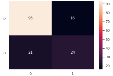
Figure 1. Confusion matrix performance of Gaussian Naïve Bayes.

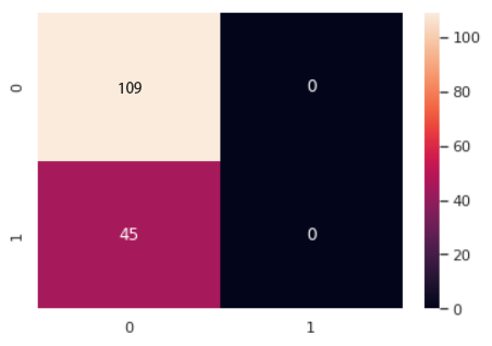
Figure 2. Confusion matrix performance of Bernoulli Naïve Bayes.

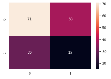
Figure 3. Confusion matrix performance of Multinomial Naïve Bayes.

The accuracy is not able to completely reflect the prediction ability of the method. This is because the wrong prediction is not just one kind. From the upper picture, it is apparently that there are three kinds of false. The accuracy is the true prediction divided by the all prediction. However, there are some false positive are included, which will cause the wrong accuracy. So, the confusion matrix enable doctor to differentiate whether a disease fit to use the method to predict. The performance of confusion matrix is demonstrated in Figure 1, 2 and 3 respectively. For diabetes, it’s a serious disease, which will cause long-time pain, even death. So, the wide range of wrong diagnostic will cause serious consequence, which is not been expected to occur by doctor. So, from the confusion matrix, it could be observed that the Gaussian Naïve Bayes has the smaller number of wrong diagnostics, while the Multinomial Naïve Bayes has the most.

Overall, synthetically, the Gaussian Naïve Bayes has the best prediction, the Bernoulli Naïve Bayes is at the mid-level and the Multinomial Naïve Bayes is the worst one.

4. Discussion

Although the performance of the Gaussian Bayes is not bad, the 70% accuracy still does not fit the demand of the Medicine. As widely known, diabetes is a serious disease. When a people, unfortunately, get diabetes, infinite cost and pain will come. The low accuracy will finally cause the wide range of wring diagnostic, which will cause catastrophic medical result. 30 percent of diabetes patients will be ignored. Simultaneously, if the technology will be used to predict another serious disease, for example the AIDS or the cancer, the requirement of the accuracy will be much higher than diabetes, maybe even over 0.99. Also, when facing such vital disease, the wide range of wrong diagnostic is definitely unacceptable. So, if this technology wants to put into use in the hospital, the optimize of the code is important and inevitable. In my opinion, the simple machine learning like the Sklearn should be optimize by the superior machine learning model, also, some deep learning should put into use, for instance the neural network, convolution neural network and deep neural network. These Deep Learning will tremendously enhance the accuracy and the true accuracy of the prediction. This is because these models are much more complex than the simple leaner machine learning model. Not just the optimization of the model, the dataset is also worth to be enriched. In the introduction, it basically introduced the type of diabetes and the aetiology of the two kinds of diabetes. The insulin and the Glucose, in fact, are important data to measure whether a people a diabetes sufferer, however, it is not enough. Some protein related to the produce of the insulin, the integrity of some gene that related to the producing of the insulin receptor and some protein related to the transform of the glucose should be included in the data of a patient. With the increasing of the dimension number, the vector will have more features, which will finally benefit the computer to make a better prediction. Also, after making the prediction, the statistic-analysis should continue. By finding the most influential factor of causing diabetes, will tremendously benefit human to prevent the happen of diabetes. This is the expectation of the future research; one step of this project will save and prevent more people falling into blackhole of diabetes.

5. Conclusion

From the result, it is easy to acknowledge that the Gaussian Naïve Bayes made the best prediction. From the accuracy, it is obviously that the Gaussian Naïve Bayes lead the accuracy and the Bernoulli Naïve Bayes tightly follow the Gaussian Naïve Bayes. However, the Multinomial Naïve Bayes only got 0.56 accuracy for its basic model may not fit to learn such kind of data. In the confusion matrix, the Gaussian Naïve Bayes still have the highest actual accuracy while the Bernoulli Naïve Bayes also predict well. The Multinomial Naïve Bayes produce falser negative and false positive than the other 2 models. So, conclusively, to make some basic prediction on some simple disease, the Gaussian Naïve Bayes and the Bernoulli Naïve Bayes is good enough to put into use. The Multinomial Naïve Bayes, because of its special algorithm, fit to figure out and clean the trash e-mail. However, if this model wants to put in use in the hospital, or even the country medical system, some high-level and complex model should use to optimize this simple model, like deep learning or neural network. All in all, this research still has a wide space for future scholar to excavate it feasibility. With the development of this model, people will make a huge progress on entire human epidemic prevention. The cure and prevention of diabetes will much easier than the time before.

References

[1]. Forouhi, N. G., & Wareham, N. J. (2010). Epidemiology of diabetes. Medicine, 38(11), 602-606.
[2]. Tao, Z., Shi, A., & Zhao, J. (2015). Epidemiological perspectives of diabetes. Cell biochemistry and biophysics, 73(1), 181-185.
[3]. Leahy, J. L. (2005). Pathogenesis of type 2 diabetes mellitus. Archives of medical research, 36(3), 197-209.
[4]. Nathan, D. M. (2015). Diabetes: advances in diagnosis and treatment. Jama, 314(10), 1052-1062.
[5]. Faiz, I., Mukhtar, H., & Khan, S. (2014). An integrated approach of diet and exercise recommendations for diabetes patients. In 2014 IEEE 16th International Conference on e-Health Networking, Applications and Services, 537-542.
[6]. Emerging Risk Factors Collaboration. (2011). Diabetes mellitus, fasting glucose, and risk of cause-specific death. New England Journal of Medicine, 364(9), 829-841.
[7]. Webb, G. I., Keogh, E., & Miikkulainen, R. (2010). Naïve Bayes. Encyclopedia of machine learning, 15, 713-714.
[8]. Mehmet, A., (2020). Diabetes Dataset. URL: https://www.kaggle.com/datasets/mathchi/diabetes-data-set
[9]. Perez, A., Larranaga, P., & Inza, I. (2006). Supervised classification with conditional Gaussian networks: Increasing the structure complexity from naive Bayes. International Journal of Approximate Reasoning, 43(1), 1-25.
[10]. Artur, M. (2021). Review the performance of the Bernoulli Naïve Bayes Classifier in Intrusion Detection Systems using Recursive Feature Elimination with Cross-validated selection of the best number of features. Procedia Computer Science, 190, 564-570.
[11]. Jiang, L., Wang, S., Li, C., & Zhang, L. (2016). Structure extended multinomial naive Bayes. Information Sciences, 329, 346-356.
Cite this article
Li,J. (2023). Estimating diabetes risk using Naïve Bayes classifiers. Applied and Computational Engineering,21,28-35.
Data availability
The datasets used and/or analyzed during the current study will be available from the authors upon reasonable request.
Disclaimer/Publisher's Note
The statements, opinions and data contained in all publications are solely those of the individual author(s) and contributor(s) and not of EWA Publishing and/or the editor(s). EWA Publishing and/or the editor(s) disclaim responsibility for any injury to people or property resulting from any ideas, methods, instructions or products referred to in the content.
About volume
Volume title: Proceedings of the 5th International Conference on Computing and Data Science
© 2024 by the author(s). Licensee EWA Publishing, Oxford, UK. This article is an open access article distributed under the terms and
conditions of the Creative Commons Attribution (CC BY) license. Authors who
publish this series agree to the following terms:
1. Authors retain copyright and grant the series right of first publication with the work simultaneously licensed under a Creative Commons
Attribution License that allows others to share the work with an acknowledgment of the work's authorship and initial publication in this
series.
2. Authors are able to enter into separate, additional contractual arrangements for the non-exclusive distribution of the series's published
version of the work (e.g., post it to an institutional repository or publish it in a book), with an acknowledgment of its initial
publication in this series.
3. Authors are permitted and encouraged to post their work online (e.g., in institutional repositories or on their website) prior to and
during the submission process, as it can lead to productive exchanges, as well as earlier and greater citation of published work (See
Open access policy for details).