1. Introduction

Deep learning has continued to make breakthroughs in the fields of speech recognition [1][2], image recognition [3][4] and natural language processing [5][6], showing great potential. With the implementation and practice of AI technology in various application fields, FinTech will also usher in a new era of intelligence. The trading platform of the banking system has a huge amount of data, and the use of deep learning algorithms to discover the gradual trend of transaction volume and make predictions, notify business personnel and system operation and maintenance personnel of possible traffic changes in advance, and provide accurate decision support for leaders is gaining more and more attention.

The open platform of a product of a bank provides secure, stable, and simple financial access services to users based on many users and access to third-party partner services [7], and the average daily transaction volume reached 8264208 (counted in 2018.04), and the users are still in a continuous growth process, as shown in Figure 1. If the minute-level prediction can be performed in advance, the abnormal transaction flow and the asymptotic trend can be detected in advance to provide decision support for the system expansion and contraction, and then reduce the system online pressure during the peak of transaction volume or release the unnecessary system resources during the low period. There are two main types of methods commonly used for time series prediction analysis, linear and non-linear. Commonly used linear algorithms include autoregressive model (AR), moving average model (MA), and autoregressive moving average model (ARMA), etc. The AR algorithm predicts the estimated value of \( {x_{t}} \) at the next moment based on a linear combination of the known previous p observations; the MA algorithm predicts the estimated value of \( {x_{t}} \) at the next moment \( \hat{{x_{t}}} \) based on a linear combination of the known forecast errors; the ARMA algorithm combines the AR algorithm and MA algorithm to predict the estimate of \( {x_{t}} \) at the next moment \( \hat{{x_{t}}} \) based on a linear combination of \( p \) autoregressive terms and \( q \) moving average terms. linear algorithms have the advantage of being simple and efficient, mainly for stable time series, i.e., the observations need to have constant amplitude on the time axis and the variance of the observations converge to the same stable value on the time axis, however, this type of algorithm has strong assumptions on the data, and the data used in this paper The data used in this paper do not have the linear relationship described above. After fitting with the above algorithm, the prediction has good results for non-special days, but there are obvious deviations for special days such as holidays, etc. However, the analysis of these special days is extremely necessary, and the trend of trading volume changes on special days of important systems is often the most noteworthy, and even its importance is far more than the usual point Therefore, the research in this paper mainly uses nonlinear algorithms. The commonly used nonlinear algorithms are autoregressive moving average (ARIMA) model, regression tree and deep neural network model. Since deep neural network has strong nonlinear function approximation ability, especially the significant advantage of long- and short-term memory network in recurrent neural network [8] in dealing with long time series prediction problem, the research in this paper is mainly based on this type of model.

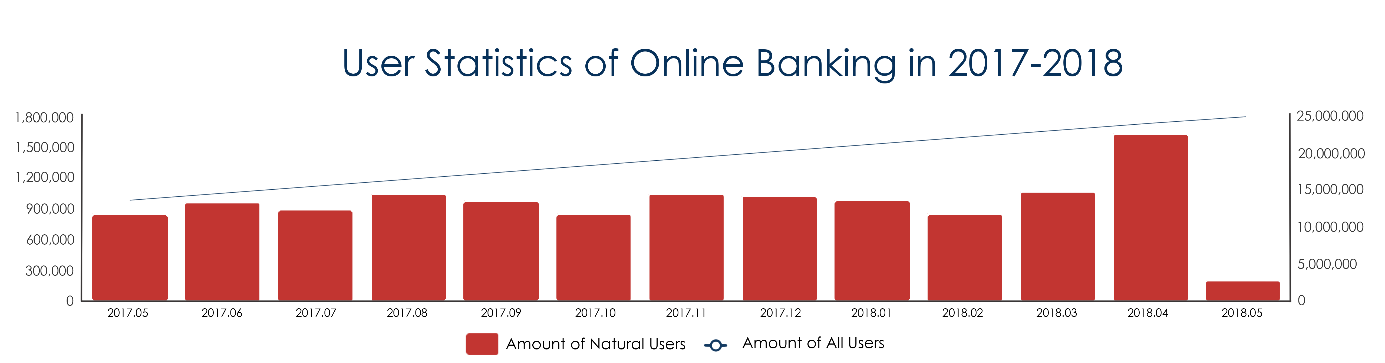
Figure 1. Online banking user growth curve.

The main research contents and contributions of this paper are as follows：

(1) To study the cyclical trends and characteristics of historical volume data, including minute level, hourly level, daily level, neighboring time sections, neighboring time regions, special days, etc.;

(2) Processing of 241 days of historical data by feature engineering, generating feature vectors of dimension [347040, 20]

(3) Design and implementation of the transaction volume prediction model LSTM-WP based on the long and short-term memory network LSTM.

(4) Training the model, hyperparameter tuning and performing comparative analysis of the prediction results, which showed that the accuracy of the LSTM-WP model on holidays was improved by about 8% compared to the linear algorithm.

2. Related technical notes

2.1. Recurrent neural networks

Recurrent Neural Network is a class of neural networks for processing sequential data. It remembers the previous information through the connection structure of nodes between each layer (also called RNN cells) and uses this information to influence the output of later nodes, This makes RNNs widely used in various fields such as speech recognition, language modeling, machine translation and temporal analysis.

The design principle of RNN is shown in Figure 2. The RNN network is expanded in the time dimension with the input \( {x_{t}} \) (the feature vector at the moment t) and, after parameterized by the weight matrix \( U \) of the input-to-hidden layer connection, the \( {h^{(t)}} \) at that moment is calculated by combining the state \( {h^{(t-1)}} \) of that node at the previous moment, as shown in Equation (1), where the hidden-to-hidden recurrent connection is parameterized by the weight matrix \( W \) parameterized by a function \( f \) denoting the activation function in the neural network.

\( {h^{(t)}}=f(U×{x^{t}}+W×{h^{(t-1)}}) \) Equation (1)

The hidden-to-output connection is parameterized by the weight matrix \( V \) . After that, the corresponding sequence of output values \( o \) is obtained from the mapping of \( x \) input sequences, and the loss function \( L \) measures the distance between each \( o \) and the corresponding training target \( y \) . The model is then trained using the back propagation algorithm and the gradient descent algorithm, and since each node at each moment has an output, the total loss of the RNN is usually the sum of all moments (or parts moments) on the loss sum. However, if the time series is too long, the RNN does not correlate this contextual information well, creating the problem of "long-term dependence", because the gradients tend to disappear (in most cases) or explode (rarely, but with a significant impact on the optimization process) after many stages of propagation [9].

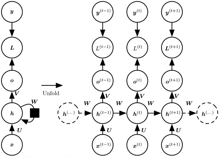
Figure 2. RNN design principle.

2.2. Long-term and short-term memory networks

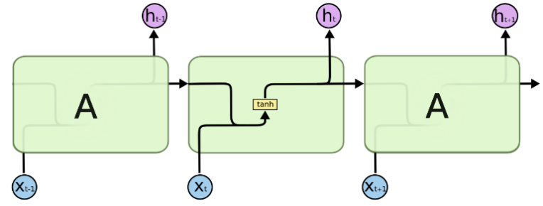
Long Short-Term Memory Network (LSTM) is a special kind of RNN, which was proposed by Hochreiter et al. in 1997 [10], mainly to solve the "long-term dependency" problem of RNN mentioned above. It replaces the original RNN cell with an LSTM cell, where the original RNN cell only applies to a single tanh loop, but the LSTM cell uses three "Gate" structures to control the state and output at different moments [11], namely forgetting gate", "input gate" and "output gate", as shown in Figure 3(a)(b). The "gate" structure here allows for selective passage of information, which is achieved using a fully connected neural network with a sigmoid activation function and a per-bit multiplication operation.

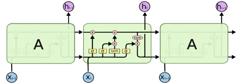
The "forgetting gate" is calculated as shown in Equation (2), which allows the LSTM cell to decide which messages to let pass. The input is \( {h_{t-1}} \) and \( {x_{t}} \) , and the output is a vector of the same length as \( {C_{t}} \) with values between 0 and 1, indicating the weight of letting each part of \( {C_{t-1}} \) pass. where 0 means that no information is allowed to pass and 1 means that all information is allowed to pass.

\( {f_{t}}=σ({W_{f}}∙[{h_{t-1}},{x_{t}}]+{b_{f}}) \) Equation (2)

The "input gate" allows the LSTM to decide which information stays in the input data at the current moment \( t. \) Its operation is divided into two steps: (1) selecting the updated information content (calculated as shown in Equation (3)) and the updated amount(calculated as shown in Equation (4)); (2) updating the cell state, calculated as shown in Equation (5) is shown.

\( {{C^{ \prime }}_{t}}=tanh({W_{C}}∙[{h_{t-1}},{x_{t}}]+{b_{C}}) \) Equation (3)

\( {i_{t}}=σ({W_{i}}∙[{h_{t-1}},{x_{t}}]+{b_{i}}) \) Equation (4)

\( {C_{t}}={f_{t}}×{C_{t-1}}+{i_{i}}×{{C^{ \prime }}_{t}}) \) Equation (5)

In the second step of the "input gate", the information that we do not want to keep is first deleted, and then the newly added information that we need to keep is added. After getting the latest node state \( {C_{t}} \) , the "output gate" combines the output \( {h_{t-1}} \) of the previous node and the input \( {x_{t}} \) of the current node to determine the output of the current node, as shown in Equation (6) and Equation (7).

\( {o_{t}}=σ({W_{o}}∙[{h_{t-1}},{x_{t}}]+{b_{o}}) \) Equation (6)

\( {h_{t}}={o_{t}}×tanh({C_{t}}) \) Equation (7)

3. Trading volume forecast

3.1. Data sets and data pre-processing

The original dataset contains a total of 241 text files from 08/27/2017 to 04/24/2018, and each text file records the number of user transactions per minute about the BOC Open Platform on that day, i.e., each text file is composed of 1440 records, so there are a total of 347,040 records.

The format of each record is: datetimetransaction volume (count)

For example: 2018-03-25 23:41:0 6015

Among these 241 text files, there are several files with records that are anomalous, such as transaction volume of 0 or transaction volume significantly different from other records in the same time period, so the outlying sample points were first processed by removing the replacement method.

3.2. Feature engineering

(1). Cyclical variation characteristics at the minute and hourly levels: Usually, the trend of the daily minute and hourly trading volume is approximately the same, as shown in Figure 4.

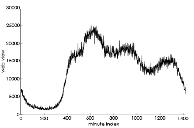
Figure 4. Volume trends at the minute and hourly levels.

(2). Cyclical change characteristics at the daily level: Usually, the change trend of trading volume for each day from Monday to Friday is roughly the same, as shown by the blue line in Figure 5, and the change trend of trading volume for Saturday and Sunday is roughly the same, as shown by the green line in Figure 5. Here, Monday through Friday are defined as working days, and Saturday and Sunday are defined as rest days.

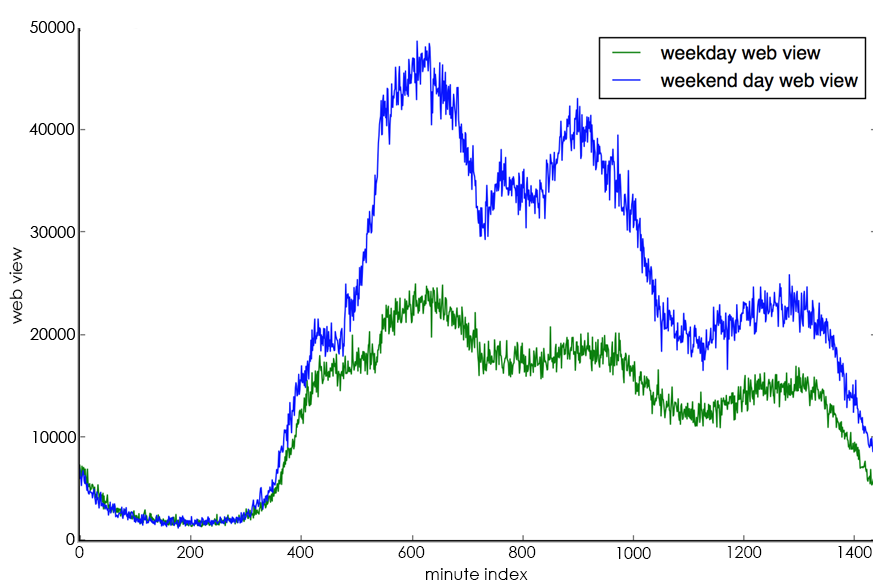
Figure 5. Trends in daily level trading volume.

(3). The characteristics of the change of trading volume in the adjacent time section: usually, if the day is a working day, then its trading volume is approximately the same as the average value of the trading volume of the 5 working days of the previous week and the trading volume of the same day of the previous week; if the day is a rest day, then its trading volume is approximately the same as the average value of the trading volume of the 2 rest days of the previous week and the trading volume of the same day of the previous week.

(4). Characteristics of the change in trading volume in the adjacent time zone: the instantaneous trading volume at the current moment is related to the change in trading volume in the period before that moment.

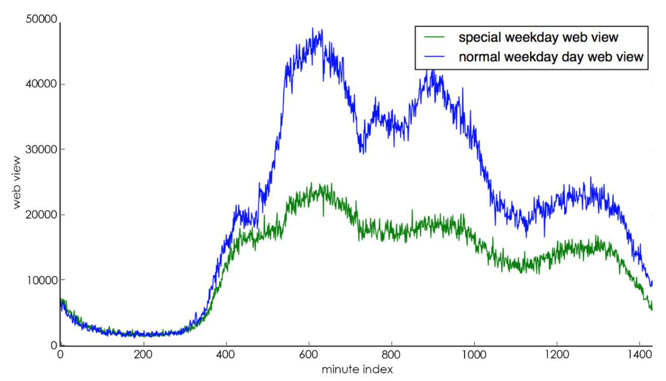
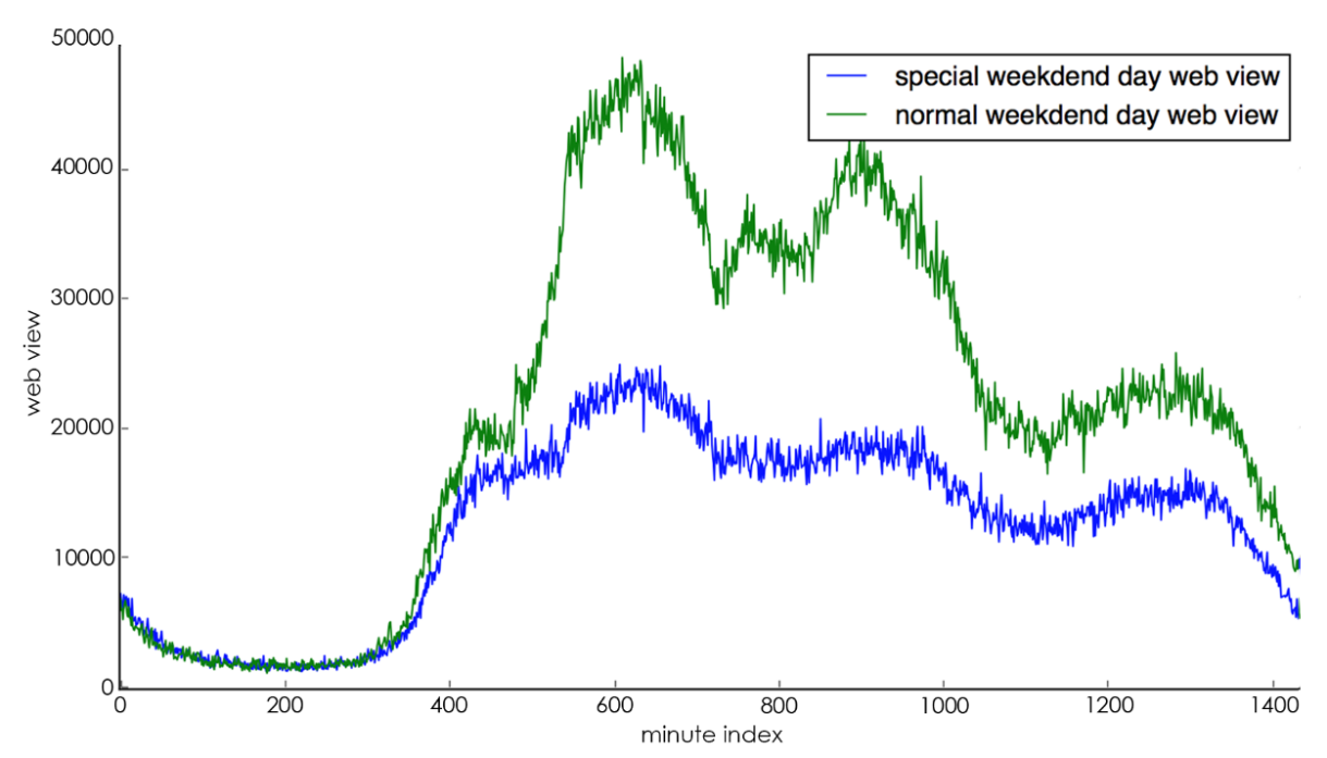
(5). The change characteristics of special days: special days include holidays (e.g., Chinese New Year, National Day, etc.), important days (e.g., major promotion days, etc.) and the dates before and after these days. The change of special days is often the opposite of the cyclical change characteristics of the day level, for example, if the day is a working day but at the same time a holiday, the trading volume of that day is usually much lower than that of other working days, as shown in Figure 6(a) shows, the blue line represents the trading volume of normal working days, and the green line represents the trading volume of special working days. It can be seen that special working days lead to lower trading volume than normal working days because the day is actually a holiday; if the day is a rest day, but at the same time it is a date that actually requires work, then the trading volume of the day is usually much higher than other rest days, as shown in Figure 6(b) As shown in Figure 6(b), the blue line represents the trading volume on a normal day off and the green line represents the trading volume on a special day off. It can be seen that a special day off leads to a much higher trading volume than a normal day off because that day is actually a working day.

Combining the above analysis, in the feature engineering stage, each record is expanded into a 20-dimensional (feature_size=20) feature vector, where the i-th record is noted as \( {X_{i}} ({X_{i}}={f_{j}},j=1,…,featur{e_{s}}ize-1 \) ) where the second feature, i.e., the transaction volume, is the focus and is noted as \( {Y_{i}} \) . The specific meaning of each dimension is shown in Table 1.

The data volume is \( 241 day×1440 minutes-time\_step=346980 \) , here time_step is taken as 60, which means every 60 consecutive minute level records as 1 sample \( {S_{i}} \) , i.e. \( {S_{i}} \) is composed of \( [{X_{0}},{X_{1}},{X_{2}},…{X_{59}}], \) so the dimension of Si is [time_step , feature_size]=[60, 20], and \( {Y_{0}} \) is the transaction volume value at the next moment, so as to generate the training and test sets, and here 90% of them are used as the training set (312282 records) and the rest of the data are used as the test set (34698 records).

Since LSTM is sensitive to the scale of the data, each dimension of the 20-dimensional features is normalized according to the nature of the features: (1) for f6 and f7 features, the value is taken as 0 or 1 using one-hot coding; (2) for other features, the z-score normalization is used to make them conform to the standard normal distribution.

3.3. Model structure

The LSTM-WP (LSTM-Webredict) model designed in this paper uses a 6-layer neural network, including Input Layer, LSTM Layer and Output Layer, as shown in Figure 7. Among them, the input transformation layer consists of 1 layer of Fully Connected Network (FCN), which is responsible for converting the training sample data \( {X_{i}} \) at each moment from the original dimension [batch_size:64, time_step:60, feature_size:20] to the same dimension as the num_units of the LSTM cell. units with the same dimensions [batch_size:64, time_step:60, num_units:128], as shown in Figure 8; the processing layer consists of 3 layers of LSTM, each layer consists of 1 LSTM cell expanded over 60 time steps (time_step), and the dropout process is added to prevent the model from over The output conversion layer consists of 2 fully connected layers, which are responsible for converting the output of the LSTM cell of the last time dimension into the predicted transaction volume, and the process of changing the data dimension is: [batch_size:64, num_units:128] -> [batch_size:64, output_layer1_ size:64] -> [batch_size:64, output_layer2_size:1], as shown in Figure 9.

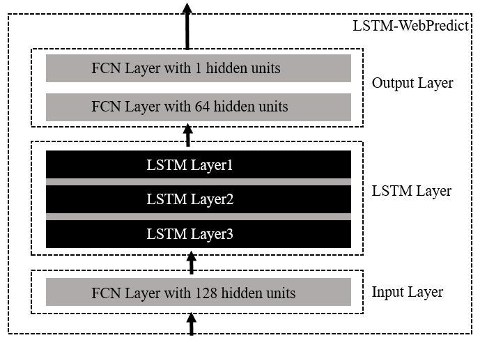
Figure 7. LSTM-WP model design.

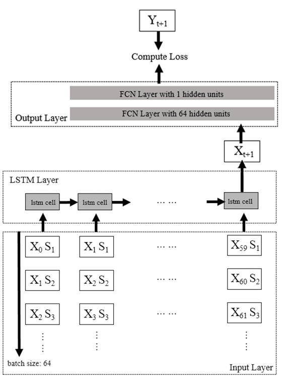
Figure 8. Input and output layers.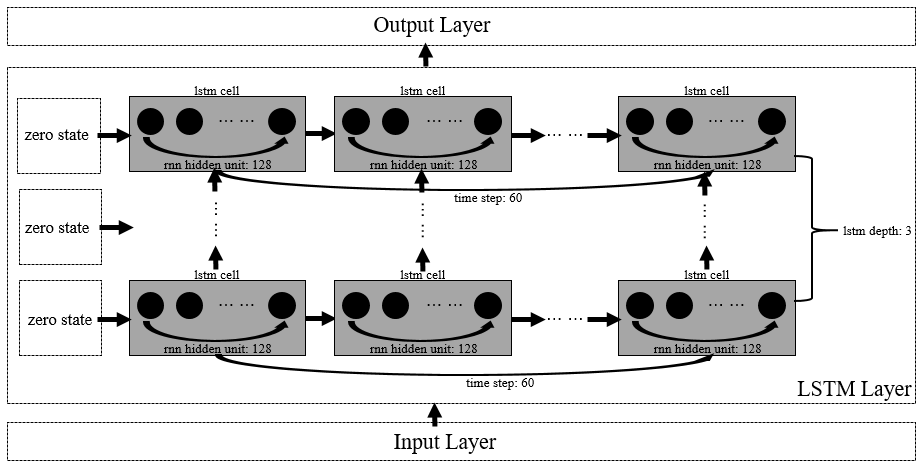

Figure 9. LSTM layer.

3.4. Training and prediction

During the training process, the model uses squared error to portray the loss and L2 regularization to prevent overfitting of the model. See Eq. (8) for the definition of the loss function and Eq. (9) for the L2 regularization formula, where \( {y_{t}} \) denotes the actual trading volume at minute \( t \) , \( {y_{pre}} \) denotes the predicted trading volume at minute \( t \) , \( γ \) denotes the regular term coefficient, \( {W_{i}} \) denotes the i-th parameter, and the model has a total of \( m \) parameters.

\( Loss=\frac{1}{2}{({y_{t}}-{y_{pre}})^{2}}+l{2_{regularizatio{n_{loss}} }} \) Equation (8)

\( l{2_{regularizatio{n_{loss}}}}=\frac{γ}{2n}\sum _{{W_{0}}}^{{W_{m}}-1}{{W_{i}}^{2}} \) Equation (9)

In the evaluation process, the model uses the root mean squared error (RMSE: root mean squared error) to evaluate the goodness of the model, which reflects the average deviation of the forecast value from the observed value, taking a value greater than or equal to zero, and is equal to zero when there is no error in the forecast. The formula for calculating the mean squared error is shown in Equation (10), where n is 1440, which indicates the 1440 minutes of the forecast day, \( {y_{t}} \) denotes the actual trading volume at minute \( t \) , and \( {y_{pre}} \) denotes the predicted trading volume at minute t.

\( RMSE=\sqrt[]{\frac{1}{n}\sum _{t=1}^{n}{|{y_{t}}-{y_{pre}}|^{2}}} \) Equation (10)

(1). In the forecasting process, this paper uses a sliding window approach to trigger the forecasting process at 0:05 a.m. each day, and to forecast the day's 1440 minutes of trading volume based on the previous day's bootstrap data and using this to continuously update the bootstrap data. The specific method is as follows, and the algorithm pseudo-code 1 gives the exact process.

(2). Generate bootstrap data: take the last 60 minutes of trading volume data of the previous day, i.e., the actual trading volume from the moment 23:00:00 to the moment 23:59:00, and generate a feature vector with dimension [time_step, feature_size];

(3). Feeding into the trained model: the model outputs the predicted value of the next moment's trading volume, such as the first trigger that generates the predicted trading volume Y0 at the 00:00:00 moment;

(4). Update the bootstrap data: use the predicted value of the transaction volume to generate a feature vector with dimension [1, feature_size] for the next moment, i.e., the feature vector for the 00:00:00 moment, and add it to the end of the bootstrap data, then delete the feature vector for the earliest moment to ensure that the bootstrap data dimension is still [time_step, feature_size];

(5). The above (2) and (3) steps are run iteratively until all 1440 minutes of the day's trading volume are predicted, i.e., from 00:00:00 to 23:59:00 of the day.

Algorithm pseudocode 1. Forecasting transaction volume based on sliding windows.

Algorithm Variable Definition:

1) lead_data indicates the lead data used to calculate the trading volume at 00:00:00 of the day

2) fv indicates the feature vector generated from the bootstrap data

3) nfv indicates the normalized feature vector

4) next_predict_count

indicates the predicted value of transaction volume at the next moment

calculated from the bootstrap data

5) predict_count indicates a sequence of 1440 volume forecasts for the day

6) next_minute_fv

indicates the feature vector for the next minute

7) lstm() indicates the trained model

8) time_from, time_to

indicates the start and end moments of the guide data

Input: time_from, time_to

Output: predict_count

Algorithm start：

1. lead_data = create_lead_data(time_from=23:00:00, time_to=23:59:00)

2. fv = create_feature_vector(lead_data)

3. nfv = normalizied(fv)

4. for i in range(1440):

5. next_predict_count = lstm(nfv)

6.predict_count.append(next_predict_count)

7.next_minute_fv = create_next_minute_feature_vector(next_predict_count)

8.fv = update_feature_vector(fv, next_minute_fv)

9.nfv = normalizied(fv)

10. Return predict_count.

3.5. Analysis of results

In this paper, the prediction results using the LSTM-WP model are compared with the prediction results of the weighted average algorithm for the Labor Day holiday period in 2018. The information on the timing of the Labor Day holiday is shown in Table 2.

Table 2. 2018 Labor day holiday information.

The corresponding prediction comparison results for the five days are shown in Table 3, which shows that the mean square error of the LSTM-WP model during the holiday period is lower than that of the weighted average algorithm by about 8.63% on average, i.e., the prediction accuracy of LSTM-WP is higher. Taking the observed data on May 1, 2018, the results are shown in Figure 10, where the red line is the prediction result of the LSTM-WP model, the blue line is the actual trading volume on that day, the yellow line is the baseline based on the LSTM-WP model (upper baseline vs. lower baseline), and the green line is the prediction result of the weighted average algorithm.

Table 3. Predicted comparison results.

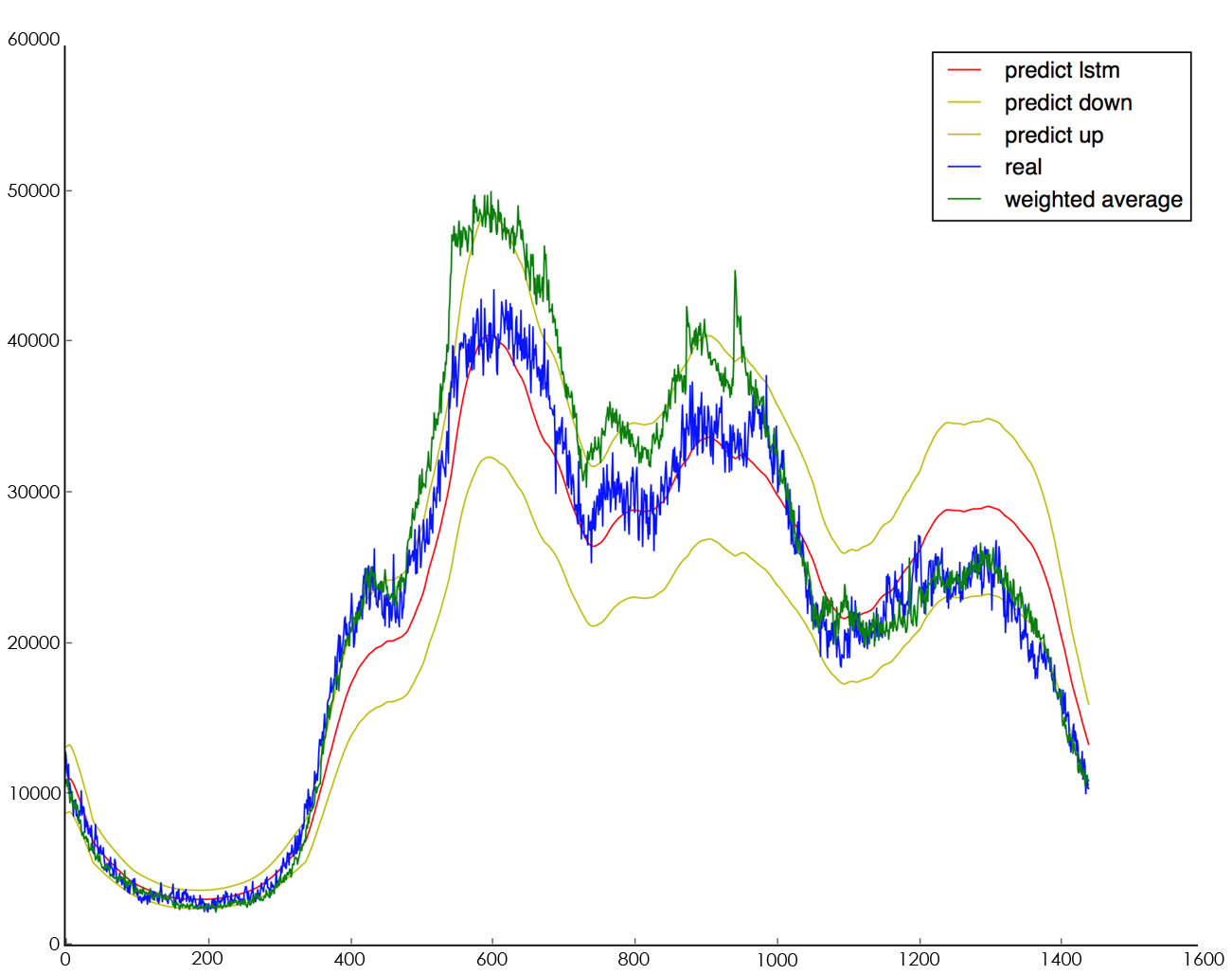
Figure 10. 2018.05.01 trading volume forecast comparison.

4. Conclusion

The contemporary landscape of fintech is witnessing a pronounced surge in the adoption of machine learning and deep learning algorithms, propelling their integration into diverse application scenarios, most notably trend prediction. In response to this evolving trend, this paper endeavors to contribute a novel and robust solution, culminating in the design and implementation of the LSTM-WP model for trading volume prediction. The foundation of this model is anchored in the formidable Long Short-Term Memory (LSTM) network, harnessed in light of an intricate analysis of historical trading volume data characteristics. This analysis serves as the bedrock for a rigorous comparative study, where the LSTM-WP model is pitted against the established statistical-based weighted average algorithm. The empirical outcomes of this study are compelling, showcasing an impressive 8% enhancement in the predictive accuracy of the LSTM-WP model, notably accentuated during the prognostication of pivotal events like special days. Intriguingly, as the volume of training data escalates, the model's learning proficiency exhibits a commendable augmentation, underscoring its adaptability and scalability. Beyond its immediate implications for trading volume prediction, this research extends its reach to a broader spectrum of time series predicaments, thereby engendering a substantial reservoir of technical expertise. In this vein, the algorithmic advancements put forth in this study serve as a catalytic force in the application of AI technology to multifarious business contexts, encompassing challenges ranging from anomaly detection to capacity assessment. In summation, this paper resonates with the emerging paradigm of leveraging machine learning and deep learning algorithms for predictive analytics within fintech. The LSTM-WP model's ascendancy in trading volume prediction, bolstered by its LSTM underpinnings, stands as a testament to the fusion of cutting-edge techniques with traditional financial domains. Furthermore, the ripple effect of this research cascades into diverse sectors, accentuating the transformative potential of AI-powered solutions across a panorama of intricate time series quandaries.

References

[1]. Dahl G E, Yu D, Deng L, et al. Context-dependent pre-trained deep neural networks for large-vocabulary speech recognition[J]. IEEE Transactions on Audio, Speech, and Language Processing, 2012, 20(1): 30-42.
[2]. Hinton G, Deng L, Yu D, et al. Deep neural networks for acoustic modeling in speech recognition: The shared views of four research groups[J]. IEEE Signal Processing Magazine, 2012, 29(6): 82-97.
[3]. Krizhevsky A, Sutskever I, Hinton G E. Imagenet classification with deep convolutional neural networks[C]//Advances in neural information processing systems. 2012: 1097-1105.
[4]. Le Q V. Building high-level features using large scale unsupervised learning[C]//Acoustics, Speech and Signal Processing (ICASSP), 2013 IEEE International Conference on. IEEE, 2013: 8595-8598.
[5]. Collobert R, Weston J, Bottou L, et al. Natural language processing (almost) from scratch[J]. Journal of Machine Learning Research, 2011, 12(Aug): 2493-2537.
[6]. Ahmed A, Aly M, Gonzalez J, et al. Scalable inference in latent variable models[C]//International conference on Web search and data mining (WSDM). 2012, 51: 1257-1264.
[7]. Bank of China opens its banking portal [EB/OL]. http://open.boc.cn/
[8]. Recurrent neural network[EB/OL]. https://en.wikipedia.org/wiki/Recurrent_neural_network
[9]. Ian Goodfellow and Yoshua Bengio and Aaron Courville. Deep learning[EB/OL]. 2016
[10]. Hochreiter S, Schmidhuber J. Long short term memory[J]. Neural computation, 1997, 9(8): 1735-1780.
[11]. Understanding- Long Short Term Memory Network (LSTMs)[EB/OL]. http://colah.github.io/posts/2015-08-Understanding-LSTMs/
Cite this article
Hu,J. (2023). A study of the transaction volume prediction problem based on recurrent neural networks. Applied and Computational Engineering,29,30-42.
Data availability
The datasets used and/or analyzed during the current study will be available from the authors upon reasonable request.
Disclaimer/Publisher's Note
The statements, opinions and data contained in all publications are solely those of the individual author(s) and contributor(s) and not of EWA Publishing and/or the editor(s). EWA Publishing and/or the editor(s) disclaim responsibility for any injury to people or property resulting from any ideas, methods, instructions or products referred to in the content.
About volume
Volume title: Proceedings of the 5th International Conference on Computing and Data Science
© 2024 by the author(s). Licensee EWA Publishing, Oxford, UK. This article is an open access article distributed under the terms and
conditions of the Creative Commons Attribution (CC BY) license. Authors who
publish this series agree to the following terms:
1. Authors retain copyright and grant the series right of first publication with the work simultaneously licensed under a Creative Commons
Attribution License that allows others to share the work with an acknowledgment of the work's authorship and initial publication in this
series.
2. Authors are able to enter into separate, additional contractual arrangements for the non-exclusive distribution of the series's published
version of the work (e.g., post it to an institutional repository or publish it in a book), with an acknowledgment of its initial
publication in this series.
3. Authors are permitted and encouraged to post their work online (e.g., in institutional repositories or on their website) prior to and
during the submission process, as it can lead to productive exchanges, as well as earlier and greater citation of published work (See
Open access policy for details).