1. Introduction

Stellar classification has been a fundamental aspect of astronomical research, providing a deeper understanding of celestial bodies and the overall structure of the universe. The Sloan Digital Sky Survey (SDSS) has brought a paradigm shift in this field, producing vast quantities of high-quality observational data and improving the way researchers study the cosmos [1]. This paper focuses on the Stellar Classification Dataset-SDSS17, a collection of 100,000 observations [2].

Notably, the dataset encompasses the class feature, specifying the classification of the astronomical object - whether it is a star, galaxy, or quasar. This mix of photometric, astronomical measurement, spectroscopic, and observational identifiers in the dataset fosters a comprehensive understanding of celestial objects, aiding in more accurate and robust stellar classification.

The objective of this research is to scrutinize the importance of these features in classifying a celestial object as a star, galaxy, or quasar, utilizing an assortment of machine learning algorithms. The classification methods used in this study include Random Forest, Gradient Boosting, and Support Vector Machine (SVM), which are well-regarded for their robustness and versatility in handling complex classification tasks [3,4]. Further, to interpret the results of these models and understand the contribution of individual features, SHapley Additive exPlanations (SHAP), an effective tool for model-agnostic interpretation, is leveraged [5].

This paper's findings will not only shed light on key features influencing stellar classification but also demonstrate the efficacy of various machine learning techniques in astronomical studies. As the field of astronomy becomes increasingly data-driven, the research will underscore the indispensable role of advanced data analysis and interpretation methodologies.

The paper is structured as follows: The "Method" section will detail the data preprocessing steps and the implementation of the classification algorithms. The "Results" section will present the output of the classification algorithms and the feature importance analysis using SHAP. The "Discussion" section will interpret these results, critically examining the implications and the interplay between various features. Finally, the "Conclusion" section will provide a summary of the findings, potential applications, and directions for future research.

This study's contribution is twofold: it employs advanced machine learning algorithms to classify celestial bodies, thereby contributing to the methodological development in the field, and it explores the significance of various observational features, enriching the understanding of the factors that influence the classification of celestial bodies.

2. Method

This section delves into the methodology employed in this research, including a brief description of the dataset used, the preprocessing steps undertaken, and the details of the machine learning algorithms and interpretation methods implemented.

2.1. Dataset

The Stellar Classification Dataset-SDSS17 utilized in this study consists of 100,000 observations of celestial bodies, each described by 17 feature columns and one class column which includes a variety of features like photometric filter data (u, g, r, i, z), right ascension and declination angles (alpha, delta), and identifiers for specific scans and fields (run_ID, rerun_ID, cam_col, field_ID. The dataset also incorporates identifiers such as obj_ID and spec_obj_ID, which uniquely classify the celestial objects in the image catalog used by CAS and optical spectroscopic objects, respectively. Moreover, the dataset contains redshift values (redshift), which offer crucial insights into the Doppler effect related to the observed celestial bodies and are essential for astronomical distance calculations and the study of cosmic expansion. Furthermore, the dataset is enriched with other observational details like the plate identifier (plate), which distinguishes each plate used in the SDSS. It also provides the Modified Julian Date (MJD), signifying the exact time of the data collection by SDSS. The fiber_ID indicates the specific fiber directing light at the focal plane in each observation. The class column categorizes the observed object as a star, galaxy, or quasar. The feature columns incorporate a mix of identifiers, angles, photometric system filters, redshift value, plate ID, Modified Julian Date (MJD), and fiber ID. A detailed description of these features can be found in the dataset's documentation. There are three target categories, namely star, galaxy, and quasar (QSR).

2.2. Data preprocessing

Prior to the application of the machine learning models, the dataset underwent a series of preprocessing steps to ensure optimal model performance. These steps included checking for missing values, dealing with outliers, and normalizing the feature values. Categorical variables were appropriately encoded to suit the machine learning algorithms.

In addition, since spec_obj_ID, obj_ID, run_ID, rerun_ID, cam_col, fiber_ID, plate and classification results are essentially irrelevant, which should be deleted when processing the classification task. And class is the classification target, which should also be deleted in the study of feature importance.

2.3. Models

Three different machine learning models are mainly selected for this study: Random Forest, Gradient Boosting, and SVM. These models were chosen for their proven capabilities in handling multi-class classification problems effectively. At the same time, simple logistic regression is also used for comparison in this research.

Random Forest: Random Forest is an ensemble learning method that operates by constructing multiple decision trees and outputting the class which is the mode of the classes output by individual trees. The function “DecisionTreeClassifier” from the sklearn is used, with the principle of Bagging integration to complete the Random Forest model with the number of decision trees set to 100, and the maximum number of features considered in each split is set to the square root of the total number of features [6].

Gradient Boosting: Gradient Boosting is another ensemble technique that builds predictive models in the form of weak learners, in a stage-wise fashion. It generalizes the model by allowing the optimization of an arbitrary differentiable loss function [7,8]. The Gradient Boosting model was implemented using the numpy and pandas, with the maximum number of weak learners to be built set to 100, the contribution of each weak learner set to 0.1, and the maximum depth of each weak learner set to 3.

SVM: SVM is a powerful algorithm for performing non-linear classification. It maps the input data into high dimensional space and finds the hyperplane that maximally separates the classes [9]. SVM with the linear kernel is implemented by sklearn.

2.4. Feature importance analysis

Performed Feature Importance analysis is also conducted on the SDSS17 dataset using the three models mentioned above.

First, for Random Forest, a node-impurity-based reduction method is used for analysis. When a feature is used to divide the data in a decision tree, the two subsets after division have lower impurity than the original dataset before division. For each feature, its average reduction is calculated in impurity over all nodes in all trees, and this total represents the importance of the feature. In general, the more the impurity is reduced, the more important the feature is. Finally, this value is normalized so that the sum of the importance of all features is 1.

Second, for gradient Boosting, the importance of each feature is calculated based on how much the feature improves the performance in each tree division in the model. The more the feature improves the prediction performance of the model (reduces the prediction error), the higher its importance.

The number of times a feature is used in a split node is calculated across all trees in the model, multiply it by the average improvement from that split, and sum it over all trees. This sum is then normalized such that the importance of all features sums to 1.

Finally, for SVMs, weight coefficients (coef_properties) are used to calculate feature importance. In a linear SVM model, each feature is assigned a weight coefficient, and these coefficients form the normal vector of the classification hyperplane. The absolute value of the magnitude of the weight coefficient of each feature can be regarded as the importance of the feature because the weight coefficient determines the degree of contribution of the feature to the classification hyperplane. The larger the absolute value of the weight coefficient, the more the feature contributes to the model and is therefore considered more important.

To interpret the results of these models and understand the influence of individual features on the predictions, the SHAP method is used, in which flow char is demonstrated in Figure 1. SHAP is a unified measure of feature importance that assigns each feature an importance value for a particular prediction [10]. It allows for high interpretability without compromising the model performance. The mathematical principle and process based on this algorithm are as follows:

\( {φ_{i}}(v)= Σ\frac{(|S|!(N - |S|- 1)!)}{N!} * [v(S ∪ \lbrace i\rbrace )- v(S)] \) (1)

where S is a feature subset that does not contain feature i, v is a value function that gives the value of a feature set in model predictions, N is the total number of features, and \( |S| \) is the number of features in the feature set S , \( v(S ∪ \lbrace i\rbrace ) \) and \( v(S) \) are the value of the feature set including feature i and not including feature i, respectively, and are usually understood as the predicted value of the model with these features.

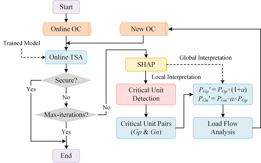
Figure 1. A flowchart illustrating the process of SHAP analysis [11].

2.5. Feature importance analysis

The performance of each model was evaluated using K-fold cross-validation, with K set to 5. This method ensures that every observation from the original dataset has the chance of appearing in the training and test set, providing a robust performance estimate.

The performance metrics used to evaluate the models were accuracy, precision, recall and F1-score. These metrics provide a comprehensive evaluation of the model performance from various perspectives.

3. Result and discussion

In this section, the author delves into a detailed analysis of the outcomes derived from machine learning models and feature importance interpretation. The performance of the machine learning models — Random Forest, Gradient Boosting, SVM and SHAP — is explored first. Subsequently, the author scrutinizes the significance attributed to different features in the process of star classification.

3.1. Result comparison

The machine learning models employed in this research offered a spectrum of classification accuracies as demonstrated in Table 1. Logistic regression is leveraged as a control. Among these, the Random Forest model exhibited the most proficient performance, achieving the highest accuracy. The performance of Gradient Boosting is usually next. And the SVM model performed the worst. Also, they all significantly outperformed the logistic regression.

Table 1. Performance comparison of various models.

Besides, the performance of the three machine learning models in the experimental group on classifying the 'star' category was superior. Among them, Random Forest and Gradient Boosting performed the best. Meanwhile, the performance of the models on classifying the 'Galaxy' category was secondary, and the performance on the 'QSO' category was the poorest.

This table elucidates the intricate differences in each model's performance, offering a broader understanding of their capabilities beyond mere accuracy. Precision, recall, and F1 score provide unique insights into the model's behavior in terms of false positives and false negatives, and the harmonic mean of precision and recall, respectively.

3.2. Feature importance analysis

To further the understanding of how these models distinguish between stars, galaxies, and quasars, a feature importance analysis was conducted using the trained models. This analysis facilitates an appreciation of which features are more instrumental in the model's decision-making process.

Interestingly, across all models, the feature 'redshift' consistently exhibited paramount importance, thereby signifying its role as a crucial differentiator in the classification task.

Table 2. Average feature importance across all models.

This figure encapsulates the average influence of each feature in the classification task, as assessed by the four models. This provides a holistic view of feature importance, discounting potential model-specific biases.

However, it is worth noting that the importance attributed to several other factors differed among the algorithms. These variations provide an interesting insight into the internal mechanisms of these algorithms, demonstrating their unique ways of leveraging information from the feature set.

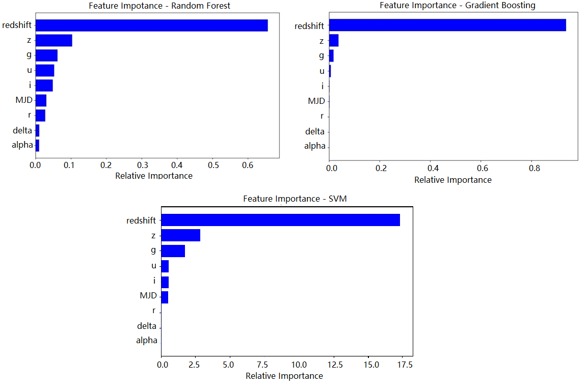
Figure 2. Feature importance of each model (Figure credit: Original).

Figure 2 provides a model-wise breakdown of feature importance, further illustrating the distinct data handling strategies employed by each model. Observing these disparities can aid in understanding model-specific biases, feature handling, and predictive power derived from each feature.

These insights on feature importance are invaluable, shedding light on how celestial measurements are utilized by machine learning models to classify an object as a star, galaxy, or quasar. These findings underscore the interplay between the features and demonstrate their collective importance in enabling accurate astronomical classifications.

The 'redshift' feature consistently exhibits significant importance across all four models, suggesting its pivotal role in celestial body classification. The considerable scores in the SVM, Gradient Boosting, and Random Forest models reinforce this finding.

The other feature importance, however, exhibits more variation between models. For example, the features 'u' and 'g' have relatively high importance according to the SHAP and SVM models, whereas the 'z' feature is more influential in the Gradient Boosting and Random Forest models. Similarly, the feature 'MJD' is identified as relatively more important in the SHAP model but is not as prominent in the other three models. These differences might be attributable to the inherent mechanisms of these models and how they handle interactions between features.

Moreover, the Gradient Boosting and Random Forest models indicate significantly high importance of 'redshift', much more so than the other features. This could be due to these models' inherent capability of handling non-linear relationships and complex interactions between features, causing them to heavily lean on this dominant feature.

In contrast, the SHAP model provides a more balanced distribution of feature importance, suggesting that, while 'redshift' is a key feature, other features also contribute to the model's predictive power. This is an advantage of the SHAP method as it considers both the main effects and interaction effects of the features, and it provides more interpretable and reliable measurements compared to traditional feature importance metrics.

In conclusion, these results emphasize the significance of the 'redshift' feature in celestial body classification tasks. However, they also indicate the necessity of considering other features for a comprehensive understanding and an effective prediction. Moreover, these results highlight the value of using multiple approaches to feature importance analysis, as different methods can shed light on different aspects of the features' contributions.

Model performance and applications

In this study, the SHAP values provide insightful interpretations of the model's performance as demonstrated in Figure 3. In particular, the 'redshift' feature is prominently influential across all classes, as confirmed by its high SHAP value. This confirms the scientific understanding of its role in astronomical object classification.

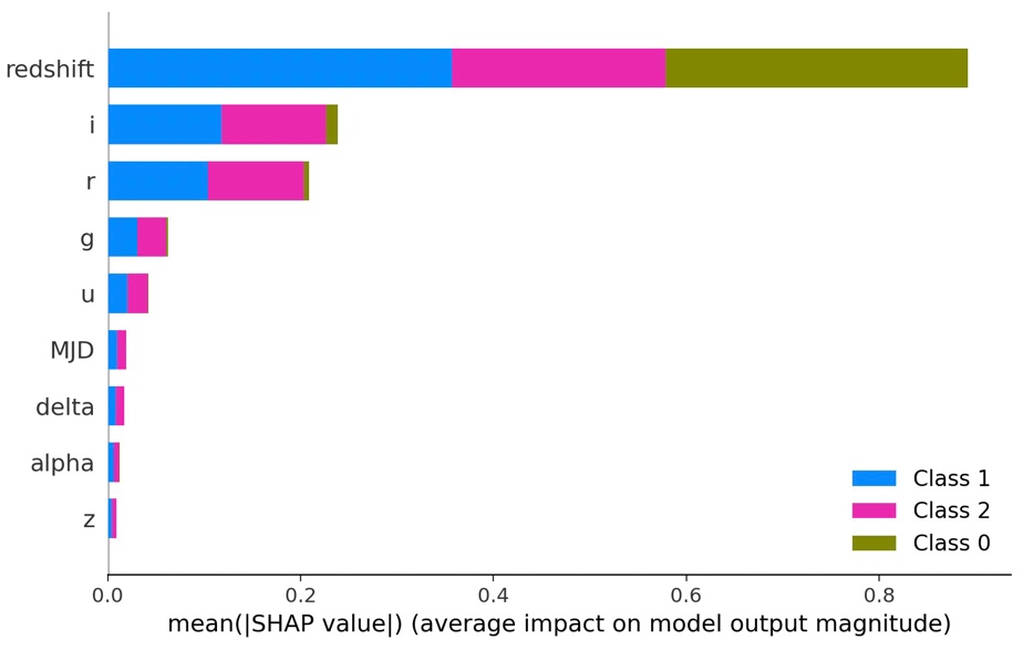
Figure 3. Average feature impact on model output magnitude (Figure credit: Original).

However, there are distinct differences among the classes. For instance, the feature importance for class ‘Star’, as indicated by SHAP values, is significantly smaller compared to classes ‘Galaxy’ and ‘QSO. This suggests that the model's predictions for class ‘star’ are less reliant on the current feature set, perhaps due to the distinct distribution or redshift playing a decisive role in the classification results of the star class. It indicates a potential area of model improvement: exploring additional features or collection of more data specifically for class ‘star’ may enhance the model performance for this class.

Lastly, while the overall consistency between SHAP values and feature importance from other methods was observed, SHAP values offer more nuanced interpretations, thus reinforcing the robustness and reliability of the findings.

Since redshift plays such an important role in the classification model, the importance of its impression on the classification results is further investigated. The redshift is bucketed, calculated the classification accuracy on each interval (using Random Forest as an example) and combined to obtain the relationship between the redshift value and the accuracy of the classification results, as shown in Figure 4. It could be found that when the redshift value is low, the accuracy is quite high. As redshift increases, the accuracy gradually decreases and achieves the lowest value at x. And then it increases again with increasing redshift. If redshift is analyzed in conjunction with the distribution density of the entire data set, it could be found that the accuracy of the model prediction and redshift are negatively correlated in the majority of the sample distribution intervals.

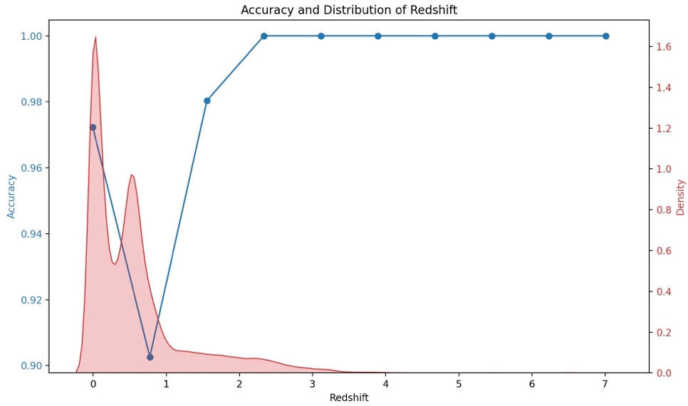
Figure 4. Accuracy and distribution of Redshift (Figure credit: Original).

4. Discussion

Given the surprising importance of the "redshift" feature, there is a need for a more in-depth study of its interaction with other features and how it affects the classification results. First, it could be noted that based on the classification results, there are only 13,716 data with negative redshift values in the dataset, accounting for 13.72% of the total data. Depending on the astronomical significance of the redshift, this may suggest the fact that the vast majority of objects are moving away from us, which perhaps serves as evidence for the universe's expanding hypothesis. On top of that, according to the Doppler effect, the result could be:

\( {λ_{observed}} = {λ_{emitted}} * (1 + z) \) (2)

Where \( {λ_{observed}} \) is the observed wavelength, \( {λ_{emitted}} \) is the original wavelength emitted by the star, and z is the redshift. This formula gives the physical definition of redshift. After performing special relativity transformation and Taylor expansion on it in sequence and keeping the first term, the result is:

\( {λ_{observed}} = {λ_{emitted}} * (1 + \frac{v}{c}) \) (3)

\( v = c*z \) (4)

Where c is the speed of light. Therefore, the velocity of a celestial body is directly proportional to the observed redshift. Just by multiplying the redshift value in the dataset by the speed of light and following similar steps for training, classifiers could be achieved based on the speed of objects or models that analyze feature importance for the speed of objects.

Similarly, according to Hubble-Lemaître law:

\( \) \( v = {H_{0}} * D \) (5)

Where H0 is the Hubble constant, and D is the distance of the star. After similar simple linear transformations, the author can also get classifiers or factor importance analysis models based on the distance of celestial objects.

This principle could also be used to explain the experimental results in 3.3. That is, the accuracy of the model prediction is very high for predicting stars very close to us, while the prediction performance is poor for medium-distance objects. And as the distance continues to increase, i.e., an earlier universe could be observed, these distant stars may have some special properties (e.g., higher luminosity, special spectral features, etc.) that allow the author to classify them more easily in a large sample, so the accuracy picks up again.

For the three algorithms, it is concluded that redshift is the most important factor affecting the star classification results, and astronomical conjectures could be made based on this. Because the redshift is positively correlated with the moving speed and distance of the celestial body, it is likely that the moving speed and distance from the Earth of the three kinds of celestial bodies, stars, galaxies and quasars, are quite different. According to the classification results, it can be guessed that most of the observed stars are very close to us, while quasars are usually very far away from the Earth.

The effectiveness of more sophisticated models, such as neural networks, could be an avenue for future exploration. However, such models were not utilized in this study due to constraints on the sample size and computational resources. Through the findings of this research and their implications, the author can envision a roadmap for future advancements in machine learning applications within the realm of astronomical research.

5. Conclusion

This research has shed light on the application of machine learning models for star classification and the relative importance of different features in such tasks. It was found that the redshift was the most influential feature by a significant margin, aligning with astrophysical theories about the universe's expansion and the role of redshift in identifying celestial bodies' distances and compositions. Moreover, the study highlighted that different models might be suitable for different tasks within astronomy, given their unique strengths and weaknesses.

Future research can explore more advanced models like neural networks and delve deeper into the interactions among features, especially the dominant redshift feature. While the current study was limited by sample size and computational resources, it nonetheless provides a stepping stone for further advancements in machine learning applications within astronomy. This research offers promising prospects for improving the efficiency and accuracy of astronomical classification tasks, thereby accelerating discoveries in the field.

References

[1]. Daud, A., Ahmad, M., Malik, M. S. I., & Che, D. (2015). Using machine learning techniques for rising star prediction in co-author network. Scientometrics, 102, 1687-1711.
[2]. Stellar Classification Dataset - SDSS17 (2022). URL: https://www.kaggle.com/datasets/fedesoriano/stellar-classification-dataset-sdss17. Last accessed: 2023/07/09.
[3]. Jordan, M. I., & Mitchell, T. M. (2015). Machine learning: Trends, perspectives, and prospects. Science, 349(6245), 255-260.
[4]. Mahesh, B. (2020). Machine learning algorithms-a review. International Journal of Science and Research (IJSR) 9(1), 381-386.
[5]. Nohara, Y., Matsumoto, K., Soejima, H., & Nakashima, N. (2019). Explanation of machine learning models using improved shapley additive explanation. In Proceedings of the 10th ACM International Conference on Bioinformatics, Computational Biology and Health Informatics, 546-546.
[6]. Rigatti, S. J. (2017). Random forest. Journal of Insurance Medicine, 47(1), 31-39.
[7]. Natekin, A., & Knoll, A. (2013). Gradient boosting machines, a tutorial. Frontiers in neurorobotics, 7, 21.
[8]. Friedman, J. H. (2002). Stochastic gradient boosting. Computational statistics & data analysis, 38(4), 367-378.
[9]. Suthaharan, S., & Suthaharan, S. (2016). Support vector machine. Machine learning models and algorithms for big data classification: thinking with examples for effective learning, 207-235.
[10]. Sahlaoui, H., Nayyar, A., Agoujil, S., & Jaber, M. M. (2021). Predicting and interpreting student performance using ensemble models and shapley additive explanations. IEEE Access, 9, 152688-152703.
[11]. Ren, J., Wang, L., Zhang, S., Cai, Y., & Chen, J. (2021). Online Critical Unit Detection and Power System Security Control: An Instance-Level Feature Importance Analysis Approach. Applied Sciences, 11(12), 5460.
Cite this article
Zhou,T. (2024). Comparison of machine learning algorithms and feature importance analysis for star classification. Applied and Computational Engineering,30,261-270.
Data availability
The datasets used and/or analyzed during the current study will be available from the authors upon reasonable request.
Disclaimer/Publisher's Note
The statements, opinions and data contained in all publications are solely those of the individual author(s) and contributor(s) and not of EWA Publishing and/or the editor(s). EWA Publishing and/or the editor(s) disclaim responsibility for any injury to people or property resulting from any ideas, methods, instructions or products referred to in the content.
About volume
Volume title: Proceedings of the 2023 International Conference on Machine Learning and Automation
© 2024 by the author(s). Licensee EWA Publishing, Oxford, UK. This article is an open access article distributed under the terms and
conditions of the Creative Commons Attribution (CC BY) license. Authors who
publish this series agree to the following terms:
1. Authors retain copyright and grant the series right of first publication with the work simultaneously licensed under a Creative Commons
Attribution License that allows others to share the work with an acknowledgment of the work's authorship and initial publication in this
series.
2. Authors are able to enter into separate, additional contractual arrangements for the non-exclusive distribution of the series's published
version of the work (e.g., post it to an institutional repository or publish it in a book), with an acknowledgment of its initial
publication in this series.
3. Authors are permitted and encouraged to post their work online (e.g., in institutional repositories or on their website) prior to and
during the submission process, as it can lead to productive exchanges, as well as earlier and greater citation of published work (See
Open access policy for details).