1. Introduction

Among the panoply of wines on offer, red wine stands out not only due to its distinctive flavor profiles but also because of its quality, which can significantly sway consumer preferences and market trends [1]. The quality of wine is a multifaceted attribute, influenced by a myriad of factors including the wine's chemical properties [2]. Gaining an understanding and making predictions about the quality of wine, especially red wine, is an important research pursuit with a wide range of practical implications in the fields of wine production, quality control, and marketing strategy.

In recent years, the deployment of machine learning techniques has broadened into various sectors, encompassing the food and beverage industry, attributed to their ability to forecast outcomes based on input data. Machine learning offers a refined and efficient method to dissect the multitude of factors influencing wine quality, thus enabling the creation of a predictive model for quality evaluation [3]. This study ventures into the convergence of machine learning and wine quality prediction. Our goal is to forecast the quality of red wine based on four crucial attributes: alcohol content, sulphates, total sulfur dioxide, and citric acid. These variables were cherry-picked due to their potent correlation with wine quality, as derived from an initial heatmap analysis. In order to achieve our research goal, applied and compared four distinct machine learning models: Logistic Regression, K-Nearest Neighbors (KNN), Decision Tree, and Naive Bayes [4]. The performance of each model was assessed, and the most dependable model for predicting wine quality was pinpointed.

2. Data used

The dataset underpinning this study is derived from the Portuguese "Vinho Verde" red wine, produced in 2009. It encompasses 1599 samples, with each sample being defined by 12 distinct attributes.

The original dataset's quality ratings, which range from 1 to 10, were preprocessed for a binary classification approach, recategorizing them into two groups: 0 indicates poor quality (original ratings 1-5), and 1 signifies superior quality (original ratings 6-10). A heatmap analysis of the dataset was executed to discern the attributes most significantly correlated with wine quality [5]. This heatmap provides a color-coded visual representation of the relationships between various wine attributes and wine quality, with the intensity of color reflecting the correlation's strength. This examination unveiled alcohol, sulphates, and citric acid as having a significant correlation with wine quality, as detailed in Figure 1.

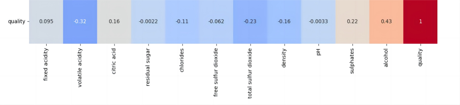
Figure 1. Heatmap of the dataset (Photo/Picture credit: Original).

While total sulfur dioxide did not stand out in the heatmap as one of the strongest correlates, included it in our analysis due to a significant finding from our grouped data. Specifically, the Table 1 displays the mean values of different parameters grouped by wine quality:

Table 1. Average values of wine attributes by quality.

The observations from this table delineate a clear pattern: wines of superior quality (quality 1) typically exhibit higher mean values for alcohol, sulphates, and citric acid, while presenting a lower mean value for total sulfur dioxide, compared to their inferior quality counterparts (quality 0) [6]. This intriguing contrast with total sulfur dioxide, despite not being listed among the top four correlations on the heatmap, provides compelling grounds for its inclusion as a predictor in the ensuing analysis. As a result, these four parameters—alcohol, sulphates, citric acid, and total sulfur dioxide—were chosen as the main focus of the study, intending to harness the power of machine learning models for predicting wine quality.

3. Proposed methodology

In the wake of the data preprocessing phase delineated in Section 2, the aim was to predict wine quality based on four attributes: alcohol, sulphates, total sulfur dioxide, and citric acid. To this end, four distinct machine learning methodologies were brought into play.

First off, Logistic Regression was put to use, a statistical method predominantly utilized for predicting binary outcomes. Owing to its simplicity and interpretability, this model set the initial benchmark for the analysis. Subsequently, the KNN method, being distance-based, enabled the classification of wine quality in accordance with the similarity of feature vectors. As the third step, a Decision Tree algorithm was set in motion. This model presented a structured, hierarchical approach to classification hinged on feature thresholds. It provided a visually enriched representation of the decision-making process. Lastly, the Naive Bayes algorithm was put into action. Despite its premise of independence among predictors, it often delivers remarkable performance, thus contributing a unique perspective to the other methods. These methodologies, selected for their distinctive properties, made the results more comprehensive and robust. Collectively, they facilitated a comparative analysis to ascertain the most effective model for predicting red wine quality. The particulars of the application of each methodology will be elucidated in the subsequent sub-sections.

3.1. Logistic regression

3.1.1. Mathematical principle

\( log(\frac{p}{1-p})= β0 + β1X1 + β2X2 + ∙ ∙ ∙ βk Xk + ϵ\ \ \ (1) \)

where, p is the probability of the dependent variable (e.g., wine quality) being 1 (e.g., high quality), and Xi are predictors (independent variables such as alcohol, sulphates, total sulfur dioxide, and citric acid). As shown in Figure 2.

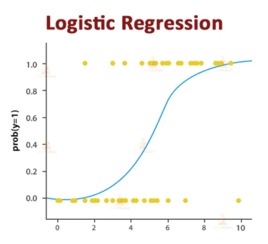
Figure 2. Logistic regression (Photo/Picture credit: Original).

3.1.2. Logistic regression implementation. This study utilizes a dataset founded on the 2009 Portuguese "Vinho Verde" red wine, encompassing 1599 samples. Each sample is defined by 12 unique attributes. The original dataset had quality ratings spanning from 1 to 10. To facilitate binary classification, these ratings underwent preprocessing, where they were grouped into two categories: 0 signifying subpar quality (original ratings 1-5), and 1 denoting superior quality (original ratings 6-10). A heatmap analysis proved instrumental in identifying the attributes most closely linked with wine quality [7]. This visual tool delineated the interrelationships between different wine attributes and the quality of the wine, with color intensity reflecting the strength of each correlation [8]. This analysis led to the identification of alcohol, sulphates, and citric acid as attributes displaying significant correlations with wine quality, as depicted in Figure 3.

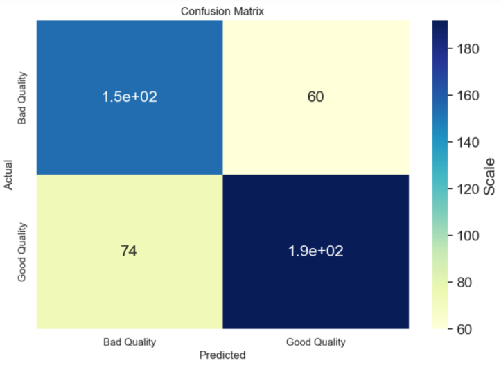
Figure 3. Confusion matrix of logic regression (Photo/Picture credit: Original).

3.2. K-Nearest neighbors

The K-Nearest Neighbors algorithm is a type of instance-based learning method widely used in machine learning. The algorithm predicts the classification of a new observation based on the classifications of its 'K' nearest neighbors in the feature space [9].

3.2.1. Mathematical principle. A KNN model can be visually and conceptually represented as : \( Classification (Z) = majority class among k nearest neighbors of Z in \lbrace X1, X2, ..., Xn\rbrace \)

Here, Z is the new instance to be classified, and X1, X2, ..., Xn are instances in the dataset, each having a class label. The 'k' nearest neighbors are selected based on a distance metric, such as Euclidean distance, in the multidimensional feature space. The classification for Z is then determined by the majority class among these 'k' nearest neighbors.

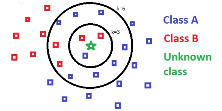
Figure 4. K-Nearest neighbors (k=3 and k=6) (Photo/Picture credit: Original).

K-Nearest Neighbors Implementation: The K-Nearest Neighbors algorithm served as the second machine learning technique utilized for predicting wine quality. The process commenced with the division of data into training and testing sets, employing Scikit-learn's train_test_split function. An 80/20 ratio was adopted for this split, designating the larger portion for training and the remaining for testing. Given KNN's dependence on the distances between feature vectors, it was essential to scale the feature values prior to KNN application. To this end, Scikit-learn's StandardScaler class was employed, performing the required standardization. The KNN algorithm was actualized using Scikit-learn's KNeighborsClassifier class, assigning the number of neighbors as 5 and employing Euclidean distance as the metric. Subsequent to training the model on the standardized training data, predictions were made on the standardized test data. Performance evaluation paralleled the method used for the logistic regression model: the calculation of an accuracy score and generation of a classification report. This report incorporated precision, recall, F1-score, and support for both wine quality categories (high and low). A confusion matrix was also formed and visualized to provide a more nuanced understanding of the model's performance. As shown in Figure 4.

The results depicted a commendable performance of the KNN model on the test data, although the accuracy score was slightly below that of the logistic regression model. The classification report suggested that the model exhibited satisfactory performance for both wine quality categories, despite occasional instances of misclassification as discerned from the confusion matrix. As shown in Figure 5.

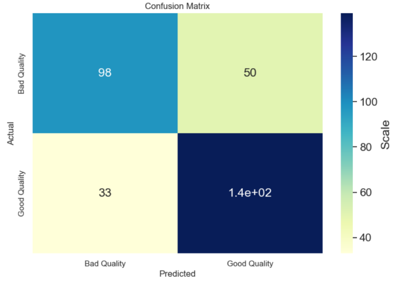
Figure 5. Confusion matrix of KNN (Photo/Picture credit: Original).

To provide a more intuitive understanding of the KNN model's operation, created a 3D scatter plot of the scaled training data, with the colors representing the actual wine quality labels. This visual representation helps to show how the KNN model uses the 'closeness' of data points in the feature space to predict the wine quality. As shown in Figure 6.

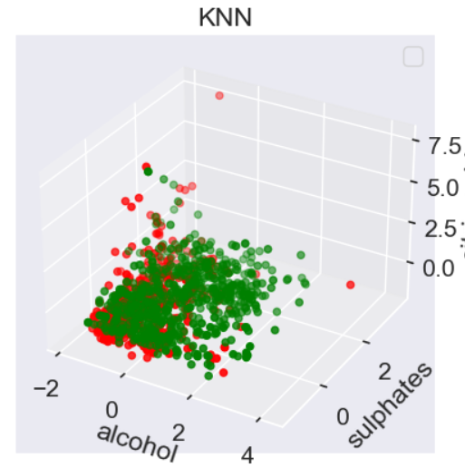
Figure 6. 3D scatter plot of KNN (Photo/Picture credit: Original).

3.3. Decision tree

A decision tree stands as a potent predictive model and is counted among the most comprehensible machine learning algorithms. Functioning in a hierarchical manner, it segmentizes the data into subsets based on varying attribute values, essentially driving decisions via specific rules and conditions [10]. Through an iterative procedure, this model continues to establish test conditions for additional attributes, further bifurcating the data. Each decision gives rise to a new branch in the tree. This process perseveres until a predefined stopping criterion is achieved, such as the exhaustion of attributes for future partitioning, or when the maximum tree depth is attained [11].

3.3.1. Decision tree implementation.The DecisionTreeClassifier class from Scikit-learn was employed to construct the Decision Tree model. The 'entropy' criterion was selected as the measure of a split's quality, serving as an indicator of the level of uncertainty or disorder within a dataset. Essentially, entropy is computed as (3).

\( Entropy = - Σ [ p(x)log2 p (x)]\ \ \ (3) \)

where p(x) is the proportion of the observations that belong to each class.

By electing entropy as the criterion, our algorithm attempts to maximize the information gain at each split. This essentially means that the model prefers the splits that yield the largest information gain. Therefore, high entropy denotes a high degree of disorder and low information gain, while low entropy signifies a well-ordered set and high information gain. As shown in Figure 7.

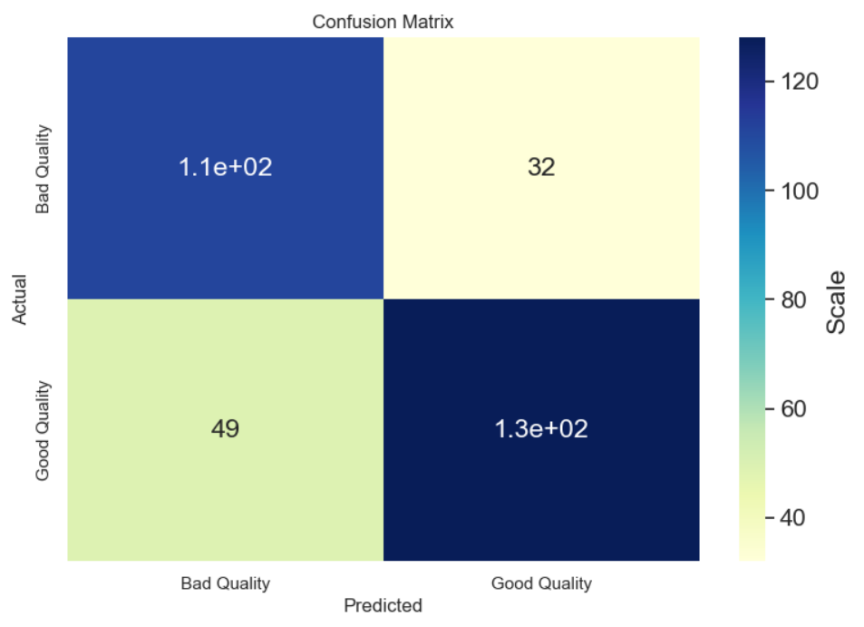
Figure 7. Confusion matrix of decision tree (Photo/Picture credit: Original).

The accuracy score of the Decision Tree model was relatively good. However, the confusion matrix revealed that there were some instances of misclassification. This suggests that the model may be overfitting the training data, which is a common problem with Decision Trees. One of the main advantages of Decision Trees is their interpretability. To leverage this, displayed the trained Decision Tree visually as a plot and as text. The plot provides a clear visualization of the decision-making process of the model, showing the conditions for each split and the distribution of classes in each leaf node. As shown in Figure 8.

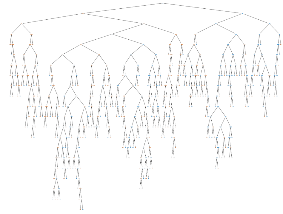
Figure 8. Decision tree (Photo/Picture credit: Original).

3.4. Naive Bayes

This algorithm calculates the probability of each category of the dependent variable given independent variables, and the prediction is made based on which category has the highest probability. Despite its simplicity and strong assumptions, Naive Bayes can be extremely effective, fast, and accurate in many scenarios [12].

3.4.1. Naive Bayes implementation. The Multinomial Naive Bayes variant was utilized, due to its effectiveness with feature vectors that are multinomially distributed.

The Naive Bayes model was initialized and trained on the designated training set utilizing the fit method. Subsequently, the model generated predictions on the test set. The model's accuracy was determined by juxtaposing its predictions on the test set against the actual wine quality classifications. This procedure culminated in the Naive Bayes model achieving an accuracy score of 60.2%, marking the lowest performance among all the evaluated models. Despite its relative simplicity, the Naive Bayes classifier did not match the performance of other models in forecasting wine quality. This may be attributed to the model's assumption of predictor independence, a condition that might not be met by the variables in this dataset. Even though the Naive Bayes model was overshadowed by other models in terms of performance, it retains value in establishing a baseline comparison for more intricate models and could potentially deliver superior results with a different set of features or hyperparameters.

Notwithstanding its lower accuracy, the Naive Bayes technique exhibited the potential of probabilistic classification models in forecasting wine quality predicated on the selected physicochemical properties. Prospective studies might delve into other variants of Naive Bayes or manipulate its parameters to bolster its predictive accuracy.

4. Conclusion

This investigation implemented four distinctive machine learning models, each yielding different insights and levels of success in predicting wine quality. The Logistic Regression model generated an accuracy of 72.08%, while KNN displayed a marginally superior outcome with an accuracy of 74.06%. Remarkably, the Decision Tree model outperformed the others, achieving the peak accuracy of 74.7%, while the Naive Bayes model fell short comparatively with a score of 60.2%.

Despite the varied accuracies, the findings suggest that machine learning can indeed function as a powerful tool within the wine industry. The ability to predict wine quality using these models has the potential to significantly optimize production processes, empowering winemakers to concentrate on the most influential variables for wine quality. This predictive capacity could also enable retailers to hone their marketing strategies and provide more precise information to consumers, culminating in enhanced customer satisfaction. Additionally, the prospect of identifying potentially subpar wines before they hit the market is a notable advantage for quality control, assisting in maintaining the high standard of wineries and preserving their brand reputation. It is crucial to recognize, however, that this investigation, as with any study, has its limitations. For example, it adopted a binary rating system for wine quality and examined only a limited set of variables. Future research could consider a more nuanced rating system for wine quality or investigate a broader range of variables impacting wine quality. Furthermore, the efficacy of other machine learning models, or even combinations thereof, could be tested for improved predictive accuracy.

References

[1]. Feher J, Lenguello G and Lugasi A. The cultural history of wine—Theoretical background to wine therapy. Cent. Eur. J. Med. 2007,2, 379–391.
[2]. Sirén H, Sirén K and Sirén J. Evaluation of organic and inorganic compounds levels of red wines processed from Pinot Noir grapes.Anal. Chem. Res. 2015, 3, 26–36.
[3]. Gupta Y. Selection of important features and predicting wine quality using machine learning techniques. Procedia Computer Science. 2018; 125:305-312.
[4]. Grewal P, Sharma P, Rathee A and Gupta S. COMPARATIVE ANALYSIS OF MACHINE LEARNING MODELS. EPRA International Journal of Research and Development (IJRD). 2022;7(6):62–75.
[5]. Reimann C, Filzmoser P, Hron, K, Kynčlová, P and Garrett, R G. A new method for correlation analysis of compositional (environmental) data – a worked example. Sci. Total Environ. 2017, 607–608, 965-971.
[6]. Al-Ghamdi A S, Using logistic regression to estimate the influence of accident factors on accident severity. Accid. Anal. Prev. 2002, 34(6), 729-741.
[7]. Bisong E. Introduction to Scikit-learn. In: Building Machine Learning and Deep Learning Models on Google Cloud Platform. Apress, Berkeley, CA, 2019.
[8]. Susmaga R. Confusion Matrix Visualization. In: Kłopotek, M.A., Wierzchoń, S.T., Trojanowski, K. (eds) Intelligent Information Processing and Web Mining. Advances in Soft Computing, vol 25. Springer, Berlin, Heidelberg, 2004
[9]. Guo G, Wang H, Bell D, Bi Y and Greer K. KNN Model-Based Approach in Classification. In: Meersman, R., Tari, Z., Schmidt, D.C. (eds) On The Move to Meaningful Internet Systems 2003: CoopIS, DOA, and ODBASE. OTM 2003. Lecture Notes in Computer Science, vol 2888. Springer, Berlin, Heidelberg, 2003.
[10]. Song Y Y, Lu Y. Decision tree methods: applications for classification and prediction. Shanghai Arch Psychiatry, vol 27, no. 2, 2015, pp.130-5.
[11]. Apté C, Weiss S. Data mining with decision trees and decision rules. Future Generation Computer Systems, vol 13, issues 2–3, 1997, pp. 197-210.
[12]. Rish I. An empirical study of the naive Bayes classifier. In IJCAI 2001 workshop on empirical methods in artificial intelligence, vol. 3, no. 22, 2001, pp. 41-46.
Cite this article
Zhan,B. (2024). Forecasting red wine quality: A comparative examination of machine learning approaches. Applied and Computational Engineering,32,58-65.
Data availability
The datasets used and/or analyzed during the current study will be available from the authors upon reasonable request.
Disclaimer/Publisher's Note
The statements, opinions and data contained in all publications are solely those of the individual author(s) and contributor(s) and not of EWA Publishing and/or the editor(s). EWA Publishing and/or the editor(s) disclaim responsibility for any injury to people or property resulting from any ideas, methods, instructions or products referred to in the content.
About volume
Volume title: Proceedings of the 2023 International Conference on Machine Learning and Automation
© 2024 by the author(s). Licensee EWA Publishing, Oxford, UK. This article is an open access article distributed under the terms and
conditions of the Creative Commons Attribution (CC BY) license. Authors who
publish this series agree to the following terms:
1. Authors retain copyright and grant the series right of first publication with the work simultaneously licensed under a Creative Commons
Attribution License that allows others to share the work with an acknowledgment of the work's authorship and initial publication in this
series.
2. Authors are able to enter into separate, additional contractual arrangements for the non-exclusive distribution of the series's published
version of the work (e.g., post it to an institutional repository or publish it in a book), with an acknowledgment of its initial
publication in this series.
3. Authors are permitted and encouraged to post their work online (e.g., in institutional repositories or on their website) prior to and
during the submission process, as it can lead to productive exchanges, as well as earlier and greater citation of published work (See
Open access policy for details).