1. Introduction

Soybeans and soybean products are very important in both daily life and the economy. They are found in many foods, like soy oil, soy milk, and tofu, and they are also a key part of animal feed for pigs and chickens. In fact, much of the meat we eat depends on soybeans first being used as animal feed. Beyond food, soybeans are also important in finance. Their prices change every day in international markets, and they are traded as futures and options. This makes soybeans both a global food source and a financial product.

What motivate us to study soybeans in the U.S.-China context are the following two reasons. First, the U.S. has long been one of the world’s largest economies and a major exporter of farm goods, resulting from its advanced agricultural technology. China, on the other hand, has relied heavily on trade to grow its economy over the past thirty years. Because of its large population and policies that limit farmland to protect forests, China depends heavily on importing farm products to feed its people. And soybeans are among the most important of these.

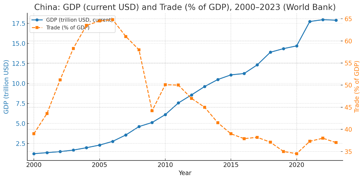
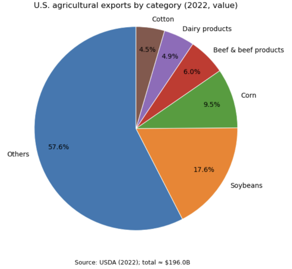
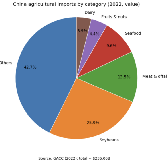
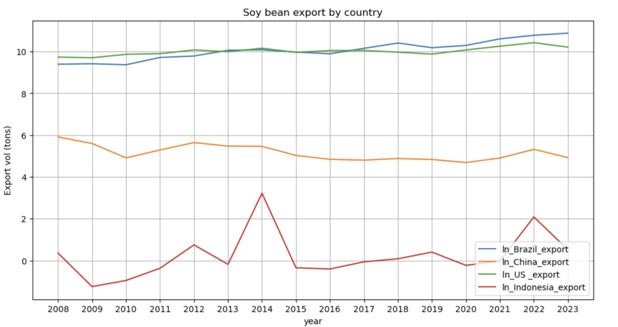
Figure 1 shows that in many years, trade has made up about 30 percent of China’s GDP, while both GDP and trade volume have grown steadily. And Figure 2 shows that soybean is the most important agricultural commodity for both China and the U.S. in terms of trade volume.

Second, since 2018, the U.S. and China have been engaged in an overwhelmingly influential trade war — the largest in recent decades. The U.S. raised tariffs on many Chinese goods from an average base level of 10% to around 30%, and China responded with tariffs on the U.S. exports to China, including soybeans [1]. Trade matters exceedingly for both economies, so these policies have serious consequences. Naturally, this raises the following questions: What are the economic and strategic reasons behind these choices? How might policies change in the future if economic conditions shift? And what kinds of policies could create win–win outcomes?

2. Analytical structure

In the global soybean market, the U.S. and China play the roles of major exporter and major buyer. To analyze their choices, we use a tool from economics called the static Nash equilibrium (NE). In this framework, each country chooses the trade volume it thinks is best, while considering how the other country might act.

To make this concrete, we divide trade volumes into three levels: small, medium, and large. For each possible combination of choices, we estimate the world soybean price using past data. We build a regression model that links world prices to trade volumes of the U.S., China, and other exporters, while also controlling for shocks like the 2008 financial crisis and COVID-19. From this, we can predict the world price for each policy choice and then calculate the economic gain or loss for both countries.

Using this payoff matrix, we find the Nash equilibrium and compare it with what actually happened in recent years. The theory predicts that the U.S. should export a low amount, while China also imports a little. But in reality, China imports a very large amount, while the U.S. follows the model’s prediction. This shows that economic costs and benefits are not the whole story.

To explain the difference, we add a “strategic benefit” for China, modeled as the natural log of its soybean imports. This reflects gains beyond short-term profits, such as ensuring food security and protecting natural forests. With this added benefit, the new Nash equilibrium matches real-world behavior: the U.S. exports a low volume, and China imports a sizable amount.

3. Literature

Soybeans are not only a basic agricultural product but also a strategic commodity that shapes international trade dynamics. Because of their role in food security and financial markets, scholars have long studied how soybean imports, exports, and prices evolve across countries. These works provide a useful backdrop for understanding today’s U.S.–China rivalry in soybeans, where trade policies and strategic choices matter just as much as supply and demand.

For example, prior research used data from 1995 to 2000 to examine China’s soybean import policies [2]. They found that China’s WTO accession and tariff reductions spurred a surge in imports, which in turn influenced global soybean prices. Similarly, other research used U.S.–China trade data from 2006 to 2016, showed how dependent U.S. soybean exports were on Chinese demand, with prices clearly shaped by trade policies [3].

Brazil has also become central in global soybean trade. For instance, research in 2015 analyzed the period 2000–2012 and concluded that infrastructure investment and better farming technology drove Brazil’s rise as the largest exporter [4]. Another research in 2017 focused on South Korea from 1998 to 2014 and studied price elasticity and food security [5]. They found that Korea was very sensitive to import price changes, but domestic reserve policies softened external shocks. In addition, a comprehensive analysis in 2004 compared the competitiveness of the U.S., Brazil, and Argentina between 1990 and 2002, highlighting exchange rates and production costs as key drivers of market share [6]. A more recent study in 2020 investigated China’s data from 2008 to 2018, showed that China deliberately reduced reliance on U.S. soybeans and diversified toward Brazil and Argentina, improving its bargaining power [7].

Overall, these studies suggest that soybean trade cannot be explained by market forces alone. Policy, infrastructure, and strategic choices all shape trade flows and prices—an insight that connects directly to our question of why China keeps importing soybeans even when the economic logic seems weak.

Game theory offers another way to analyze these issues by focusing on the strategic interactions between countries. In bulk commodity markets, exporters and importers constantly adjust their behavior based on what they expect the other side to do. This approach helps explain not just the economics of soybean trade, but also the political strategies behind it.

For instance, studies on the coffee market from 1970 to 2000 found that export quotas implemented by major producers such as Brazil and Colombia significantly influenced world prices, although long-term cooperation among exporters proved fragile [8]. Similarly, analyses of China’s rare earth export restrictions from 2005 to 2014, using a non-cooperative game framework, revealed that such policies enhanced China’s pricing power in global markets [9]. In addition, research on rice exports from Thailand and Vietnam between 1980 and 2005 concluded that intense competition between the two countries exerted sustained downward pressure on international prices [10].

Turning back to soybeans, several studies have examined U.S.–China interactions during the 2010–2018 trade war. Evidence suggests that while tariffs imposed by both sides harmed their economies, China mitigated part of the damage by diversifying its import sources [11]. From a theoretical perspective, researchers have developed a dynamic game model using data from 2008 to 2019, showing that China is willing to pay a price premium to secure long-term food supply stability [12]. Furthermore, analyses of Brazil and Argentina between 2015 and 2020 explored the feasibility of coordinated soybean export policies, though domestic political and economic conflicts ultimately hindered such cooperation [13].

These works confirm that game theory is well suited to capturing the tension between economic payoffs and strategic motives in commodity trade. For soybeans, the key takeaway is that China’s large-scale imports are not simply about minimizing cost—they are also about maximizing long-term security and bargaining power. This perspective sets the stage for our own Nash equilibrium framework, which highlights how strategic benefits can outweigh narrow economic calculations.

4. Data

Agricultural trade exhibits pronounced cyclicality and vulnerability, driven by both global supply-demand fundamentals and influenced by international logistics, geopolitical risks, and macro-financial conditions. As a vital category for both human consumption and animal feed, the prices and trade flows of this commodity directly impact food security and inflation formation. In this section, we first briefly review the production-related price aspects of soybeans in both countries and then give an overview of the international soybean market.

We rely on a combination of trade and price data. Annual import and export values are drawn from Observatory of Economic Complexity (OEC), while global price series comes from MacroTrends. These data were manually collected year by year and then merged for consistency. All import values are converted to U.S. dollars, and log transformations are applied in Figure 4 and the regression analysis to make the scale comparable and coefficients interpretable in terms of elasticity.

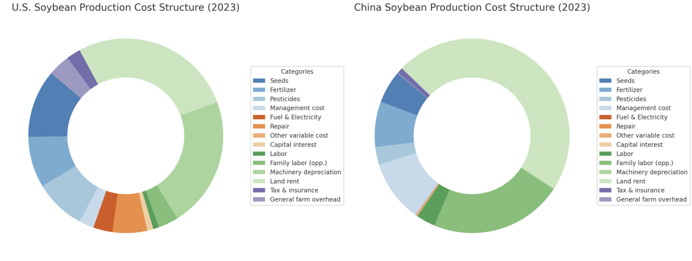
Before turning to trade flows, it is useful to compare production costs in the two countries, since these costs directly shape competitiveness in international markets. Figures 3 provides pie charts of soybean production costs in the U.S. and China. For the U.S., costs are spread across seeds, fertilizer, fuel, labor, and equipment, with mechanization keeping labor relatively low. In China, however, labor and land rent take up a larger share, reflecting differences in farming practices and land use. These comparisons give us a basic reference point for understanding why U.S. soybeans tend to be cheaper in world markets, while China relies more on imports.

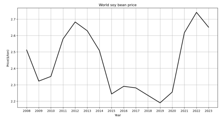
Looking at the overall time series, we see that major exporting countries entered a steady growth phase in soybean exports around 2010, with two clear peaks in 2011–2013 and 2021–2022. These peaks coincide with global shocks and cyclical rises in world soybean prices. Importantly, not all economies responded the same way: some countries sharply reduced imports during price surges, while others-maintained demand due to national strategies or inelastic needs. For our study, this highlights how world price movements can trigger very different behaviors across countries—and why China’s persistent high imports stand out as a strategic choice, not just a price-driven one.

The data also reveal resilience patterns during global crises. In the 2008–2009 financial crisis, most economies saw synchronized slowdowns, though recovery paths varied. In contrast, during the COVID-19 pandemic (2020–2022), import fluctuations were more pronounced, linked to logistics bottlenecks and shipping costs. Some countries showed quick “V-shaped” rebounds, while others plateaued with stable but lower trade. For China, the ability to sustain imports even during disruption underlines its policy-driven commitment to food security—an element our later game-theoretic framework needs to account for.

In terms of exporter market share, Brazil and the U.S. dominated global supply, while emerging players such as China, Australia, and Russia steadily increased their role in imports. These shifts reflect not only production capacity but also deliberate trade agreements and adjustments in sourcing. From China’s perspective, diversifying imports away from the U.S. toward Brazil and Argentina increased its bargaining power. This shift is directly relevant to our model, where import strategies are shaped not only by cost but also by strategic positioning in the world market.

Finally, the global price–trade relationship shows that higher prices often correlate with higher imports, but in a non-linear way. Some countries increased imports despite rising costs—likely due to stockpiling or policy-driven reserves—while others reduced demand. This heterogeneity suggests that price alone cannot explain trade behavior. For China, maintaining high imports even at elevated prices reflects strategic motives: ensuring food security, stabilizing livestock production, and protecting against supply shocks. This connects directly to our Nash equilibrium model, where adding a “strategic benefit” term helps reconcile theory with observed reality.

5. Model

5.1. Model setup

We build a simple model to study the soybean trade between the United States and China. The first step is to construct a static NE matrix as in Table 1. This matrix lists all the possible strategies of the two countries. The U.S. can choose to export at a high, medium, or low level, while China can choose to import at a high, medium, or low level. In each case, both countries get a payoff denoted by  $$ Z$$ . By comparing these payoffs, we can find the NE strategy and then check if it matches the real-world pattern of soybean trade.

To calculate payoffs, we first define China’s payoff as the cost of importing plus an extra “strategic bonus” from protecting farmland and securing food supply. Denote the payoff of two countries by  $$ Z_{country}$$ , where

$Z_{CN}=-P_{world}(I_{CN},E_{US})\ast I_{CN}\text{}+\varphi \ast ln\text{⁡}{I}_{CN},Z_{US}=P_{world}(I_{CN},E_{US})\ast E_{US}\mathrm{.}$

In the expressions,  $$ P_{world}$$  is a function of China’s import,  $$ I_{CN}$$ , and the export by the U.S.,  $$ E_{US}$$ . In addition,  $$ \varphi $$  is a parameter whose range is to be determined by comparing the theoretical NE with what happens in practice. Moreover, since the static NE we use is a discrete version of the real trade flow, we set  $$ I_{CN} $$ and  $$ E_{US}$$  to be the 25%, 50%, and 75% percentile of the two countries’ trade volume in the past 15 years.

One may wonder why China’s strategic bonus is defined as  $$ \varphi \mathrm{ }*\mathrm{ ln}{I}_{CN}$$ . Here are two major concerns that draw our attention when we develop this model. First, if assume the gain to be just  $$ \varphi \mathrm{ }*I_{CN} $$ , i.e., without the natural logarithm, China’s total payoff can be simplified to  $$ Z_{CN}= I_{CN}\mathrm{ }*$$  ( $$ \varphi $$  –  $$ P_{world})$$.

As long as  $$ \varphi $$  >  $$ P_{world}$$ , the more China imports, the higher the payoff is. This would encourage China to always import as many as it could, because the payoff would rise unboundedly. But in fact, we see that China’s importing volume fluctuates year by year, which contradicts with what  $$ \varphi \mathrm{ }*I_{CN}$$  would predict. Hence, mathematically we need to make the strategic payoff to have diminishing return. Economically, this is also reasonable because the forests to protect and the domestic consumption gap in China have natural upper bounds, therefore China would be incentivized to only import a reasonable amount rather than infinity.

Second, with diminishing return, we could have used a quadratic term instead of a natural logarithm. The latter is preferred because the quadratic coefficient must be negative to induce concavity, which would make China’s total payoff to be even more negative. However, we hope to obtain a positive return as an implicit assumption in the payoff is to be positive for economic reasons: otherwise, a country could have imported nothing and achieve a zero payoff that is better than suffering the importing cost plus strategic gain.

The next step is to estimate the relationship between world price and how the two countries (as well as other major market participants) behave. We decide to use a multivariate linear regression of the following form:

$ln\text{⁡}{Y}_t={\beta }_0+{\beta }_1\times ln\text{⁡}{I}_{CN,t}+{\beta }_2\times ln\text{⁡}{X}_{USEX,t}+{\beta }_3\times ln\text{⁡}{X}_{BrazilEX,t}+{\beta }_4\times ln\text{⁡}{X}_{UkraineEX,t}+{\beta }_5\times ln\text{⁡}{I}_{JapanIM,t}+{ϵ}_t,$

where  $$ Y_t$$  is the world price in year t, and the five regressors are the natural logarithms of China’s import, the export by the U.S., Brazil, and Ukraine, and Japan’s import respectively. The last three countries are picked as controls as they are constantly the top traders in the world soybean markets. And since the sample we use only has 16 years from 2008 to 2023, hence we cannot include as many regressors as we wish for the purpose of  $$ p<n$$ . In the actual regression we estimate, a control for COVID-19 is also included.

Before demonstrating the regression results, we want to emphasize two critical points that motivate us to employ multivariate linear regression in this setting.

First, prices are mostly driven by demand and supply. Hence to predict price fluctuations, as long as the predictor set contains import and export in trade scenario, that would be able to capture most of the price variations in the time domain. And given the sample limit of only around 16 data points, a linear regression is appropriate for this prediction task.

Second, the coefficients from the linear regression can help us check if the model makes economic sense. Since we use natural logarithms for both the outcome variable and the explanatory variables, the beta coefficients can be interpreted as elasticities. For β₁, we expect it to be positive, because when China imports more, the demand curve shifts to the right and the world price should increase. For β₂, we expect it to be negative, because when the U.S. exports more, the supply increases and the world price should decline. With this economic logic, we can see whether the estimated regression matches our expectations. It is important to note that we are not making a causal claim here. Instead, we are only looking at correlations between supply or demand and the price response, and this correlation is enough for our purpose of a sanity check.

5.2. Model results

Table shows how different countries’ soybean trade and the COVID dummy affect the world soybean price. Here we mainly focus on China and the U.S.

For China’s imports, the coefficient is 0.8449, which means if China imports 1% more soybeans, the world price goes up by about 0.84%. This is positive, and it matches economic logic: higher demand pushes the price up. For U.S. exports, the coefficient is -1.3791, which means if the U.S. exports 1% more soybeans, the world price falls by about 1.38%. This is negative, and also matches economic logic: higher supply pushes the price down.

The COVID coefficient is positive (0.1899), which makes sense because food shortages during the pandemic could raise world food prices, including soybeans. The R² is 0.767, meaning about 77% of the changes in world soybean price can be explained by just a few predictors. This is quite high given the small number of variables, so the model is useful for prediction. Since our goal is prediction, we do not need to focus on the adjusted R².

Overall, the key coefficients for China and the U.S. are in the expected directions, which shows that the model is consistent with economic reasoning. And because the R² is strong, the regression is good enough to be used for our payoff calculation in the NE analysis.

Based on the estimated regression results, we take the discretized strategies of

China and the U.S. and plug them into the regression to get the world soybean price under each case. Then, we use this predicted price in the payoff equations

of both countries. For China, we do not include the strategic gain at this stage. In this way, we can fill in the whole Nash Equilibrium matrix.

In Table 3, the yellow cells mark the U.S. best choices, and the green cells mark China’s best choices. The Nash Equilibrium without China’s strategic gain is found at China choosing low imports and the U.S. choosing high exports. However, this does not fit the reality we observe, because in the past few years China has been importing at a high level. This mismatch tells us that we cannot ignore China’s strategic gain. It plays a key role in explaining why China still chooses high imports in practice.

Our next step is to find a range where China's strategic response results in a new NE: China imports heavily while the U.S. exports little. Since the U.S. always prefers exporting less—raising soybean prices—we only need to ensure that China chooses high imports when low U.S. exports are certain. Mathematically, this means:

$Z_{CN}^{High}=max(Z_{CN}^{High},Z_{CN}^{Mid},Z_{CN}^{Low})$

Now plug in the payoff expressions to yield the following inequalities:

$$$ -P_{world}(I_{CN}, E_{US}\mathrm{ })\mathrm{ }\mathrm{*}\mathrm{ }{I}_{CN}^{High}\mathrm{}\mathrm{ }+\mathrm{ }\varphi \mathrm{ }\mathrm{*}\mathrm{ ln}{I}_{CN}^{High}>-P_{world}(I_{CN}, E_{US}\mathrm{ })\mathrm{ }\mathrm{*}\mathrm{ }{I}_{CN}^{Mid}\mathrm{}\mathrm{ }+\mathrm{ }\varphi \mathrm{ }\mathrm{*}\mathrm{ ln}{I}_{CN}^{Mid}$$$

$$$ -P_{world}\left(I_{CN}, E_{US}\mathrm{ }\right)\mathrm{*}{I}_{CN}^{High}\mathrm{}\mathrm{ }+\mathrm{ }\varphi \mathrm{ }\mathrm{*}\mathrm{ ln}{I}_{CN}^{High}>-P_{world}(I_{CN}, E_{US}\mathrm{ })\mathrm{ }\mathrm{*}\mathrm{ }{I}_{CN}^{Low}\mathrm{}\mathrm{ }+\mathrm{ }\varphi \mathrm{ }\mathrm{*}\mathrm{ ln}{I}_{CN}^{Low}$$$

$$$ -P_{world}(I_{CN}, E_{US}\mathrm{ })\mathrm{ }\mathrm{*}\mathrm{ }{I}_{CN}^{Low}\mathrm{}\mathrm{ }+\mathrm{ }\varphi \mathrm{ }\mathrm{*}\mathrm{ ln}{I}_{CN}^{Low}>0$$$

Substituting in the estimated world price and the discretized value of the trade volume by two countries, eventually we get:  $$ \varphi >54294.1$$ .

Assume  $$ \varphi =54295$$, the matrix becomes the following and now our theoretical prediction now matches the reality.

6. Conclusion and discussion

This paper uses a static Nash Equilibrium (NE) model to study the price–quantity game between China and the U.S. in soybean trade. The model shows that if we only look at costs and prices, China’s best choice should be to import a low number of soybeans. But in reality, China has kept importing a high amount over the past few years. This gap means that the simple price–cost logic is not enough to explain a country’s behavior in bulk agricultural products. Based on past studies and data, we can see that China’s soybean import decision is strongly driven by strategic reasons, such as protecting food security, stabilizing domestic prices, and ensuring the supply chain for animal feed.

This finding has two important lessons. First, when we analyze trade in major commodities, we cannot only think about static efficiency or market balance. We also need to consider strategic factors. Soybeans are not only a consumer good but also a strategic material. Their import and export volumes directly affect food security and overall economic stability. Second, from a global view, the soybean game between China and the U.S. not only changes trade patterns between the two countries but also affects other big exporters, such as Brazil and Argentina. This in turn reshapes how global soybean prices are set. This means that if future policies are designed only around short-term price changes, they may miss the long-term issues of security and strategic competition.

References

[1]. Benguria, F., Choi, J., Swenson, D. L., & Xu, M. J. (2022). Anxiety or pain? The impact of tariffs and uncertainty on Chinese firms in the trade war. Journal of International Economics, 137, 103608.
[2]. Carter, C. A., & Lohmar, B. (2002). Regional restrictions on agricultural import patterns: The case of China’s soybean imports. Agricultural Economics, 27(3), 321–330.
[3]. Lia, H., Zhang, Y., & Wang, C. (2018). Dependency and volatility in Sino-US soybean trade: A policy-driven analysis. Journal of International Trade & Economic Development, 29(4), 456–472.
[4]. De Souza, M., & Garcia, R. (2015). Infrastructure, technology and export expansion: The case of Brazilian soybeans. World Development, 70, 1–14.
[5]. Kim, S., & Lee, J. (2017). Price elasticity and food security: South Korea’s soybean import policy. Asian Journal of Agriculture and Development, 14(2), 89–104.
[6]. Marchant, M. A., Koo, W. W., & Hart, C. E. (2004). International trade and competition in soybean markets. Journal of Agricultural and Applied Economics, 36(1), 121–134.
[7]. Wang, Y., & Wang, L. (2020). Diversifying import sources: China’s strategy to enhance bargaining power in soybean markets. China Agricultural Economic Review, 12(3), 511–528.
[8]. McCorriston, S., & MacLaren, D. (2007). Cooperation and competition in coffee export quotas: A game theory approach. Journal of Agricultural Economics, 58(2), 225–241.
[9]. Huang, J., & Chen, W. (2015). Export restrictions and pricing power in rare earth markets: A non-cooperative game analysis. Resources Policy, 46, 12–20.
[10]. Ito, S., & Peterson, E. W. (2010). A duopoly model of rice export competition: Thailand and Vietnam. Agricultural Economics, 42(2), 187–196.
[11]. Liu, X., & Yue, C. (2019). Game analysis of Sino-US soybean trade friction: Welfare effects and strategic responses. Journal of Global Economic Analysis, 4(2), 78–95.
[12]. Zhang, R. (2021). Food security and import strategy: A dynamic game analysis of China’s soybean trade.
[13]. Johnson, M., & Brožena, K. (2020). Coordination challenges in a potential South American soybean export alliance: Evidence from Brazil and Argentina. International Economics and Economic Policy, 17(3), 567–585.
Cite this article
Lu,X.;Min,J.;Huang,Y.;She,Y. (2025). Soybeans at the Center of U.S.–China Trade: A Nash Equilibrium Approach. Advances in Economics, Management and Political Sciences,244,1-10.
Data availability
The datasets used and/or analyzed during the current study will be available from the authors upon reasonable request.
Disclaimer/Publisher's Note
The statements, opinions and data contained in all publications are solely those of the individual author(s) and contributor(s) and not of EWA Publishing and/or the editor(s). EWA Publishing and/or the editor(s) disclaim responsibility for any injury to people or property resulting from any ideas, methods, instructions or products referred to in the content.
About volume
Volume title: Proceedings of ICFTBA 2025 Symposium: Strategic Human Capital Management in the Era of AI
© 2024 by the author(s). Licensee EWA Publishing, Oxford, UK. This article is an open access article distributed under the terms and
conditions of the Creative Commons Attribution (CC BY) license. Authors who
publish this series agree to the following terms:
1. Authors retain copyright and grant the series right of first publication with the work simultaneously licensed under a Creative Commons
Attribution License that allows others to share the work with an acknowledgment of the work's authorship and initial publication in this
series.
2. Authors are able to enter into separate, additional contractual arrangements for the non-exclusive distribution of the series's published
version of the work (e.g., post it to an institutional repository or publish it in a book), with an acknowledgment of its initial
publication in this series.
3. Authors are permitted and encouraged to post their work online (e.g., in institutional repositories or on their website) prior to and
during the submission process, as it can lead to productive exchanges, as well as earlier and greater citation of published work (See
Open access policy for details).