1. Introduction

The Chinese commodity market has experienced remarkable growth and development, attracting increasing attention in recent years. Consequently, there is a growing interest in developing trading strategies specifically tailored for this market. Previous studies have focused on trading strategies based on technical analysis, machine learning, and statistical arbitrage. Portfolio construction, along with various weighting methods and risk management techniques, has also been explored. Despite the progress made in this area, there is still considerable room for improvement, particularly in incorporating fundamental analysis and enhancing the robustness of trading strategies.

Breakouts occur when the price of a commodity moves beyond an established trading range. This strategy involves taking a long position when the price breaks above resistance and a short position when the price breaks below support. There are two significant motivations behind this approach: (1) capturing market momentum and (2) exploiting increased volatility and liquidity of domestic commodity futures resulting from a surge in transactions. The profitability of simple moving averages and trading range breakouts in Asian stock markets served as the inspiration for this strategy [1].

Economic Intuition

When a commodity's price surpasses a defined price level, it typically leads to increased volatility, and prices tend to continue in the direction of the breakout. These breakouts are considered the starting point for subsequent increases in volatility, large price swings, and significant price trends. To elaborate further, as the price of a commodity moves beyond its normal trading range, market participants begin entering long and short positions to capitalize on perceived opportunities. This heightened market participation amplifies volatility, and intense buying and selling accelerate unstable market conditions, resulting in more significant price fluctuations. Consequently, the likelihood of a strong trend emerging becomes more probable.

Signal Generation

The signal for this strategy will be calculated as the difference between the price and the moving average, divided by a fixed number of standard deviations. The moving average represents an average price that is continuously updated and reflects the trend direction of a contract. The standard deviations aim to capture the volatility within a specified period. The moving average plus the standard deviation represents the resistance level for a range breakout, while the moving average minus the standard deviation represents the support level [2].

Portfolio Construction

The portfolio will be constructed using signal weighting methods. However, since trades are not entered simultaneously, we assign a unit value to each position and adjust it based on the calculated signals. Positions will be long for contracts with signals higher than one, short for contracts with signals lower than -1, and closed when the price touches the moving average. Additionally, a stop-loss level will be implemented to prevent substantial losses resulting from false signals [1].

Performance Estimate

Given the lack of available data on trading commodity range breakouts, we refer to the performance of this strategy in the Taiwan stock market to estimate the associated risk and return [2]. It is generally believed that commodity prices are more likely to continue in the direction of breakouts compared to securities. Consequently, profitability should be higher, and volatility should be lower in commodity markets due to the reduced likelihood of false breakouts [3].

Key Performance Metrics

Annualized Return: 10%

Annualized Volatility: 16%

Sharpe Ratio: 0.5

We apply the range breakout strategy to the commodity market and construct our portfolios accordingly.

This study develops a trading strategy for the Chinese commodity market based on the economic intuition that breakouts from defined price levels serve as the starting point for subsequent increases in volatility, large price swings, and significant price trends. The strategy utilizes the difference between the price and the moving average, divided by a fixed number of standard deviations, as a signal. The portfolio is then constructed using signal weighting methods.

2. Specification & Robustness Test

2.1. Research Method

2.1.1. Economic Intuition

The underlying economic intuition suggests that when a commodity surpasses an established price level, it induces panic among complacent short-sellers, leading them to buy-cover their positions. Simultaneously, this price movement attracts prospective buyers. The surge in panic buying creates a demand that exceeds the existing supply, resulting in a spike in prices to new highs. Increased market participation also intensifies volatility and contributes to unstable market conditions, amplifying the magnitude of price fluctuations. Consequently, the initial bullish price breakthrough evolves into a sustained upward trend.[4]

*It is important to note that a genuine breakout must be accompanied by a surge in trading volume, as heavy volume serves as a crucial indicator of conviction and interest. Therefore, the price is more likely to continue moving in the direction of the breakout.

To evaluate the effectiveness of our trading strategy, we will utilize the following statistical measures:

2.1.2. Return

1. Annualized Return:

\( Annualized Return=Log（Sum of R daily)* 250 \)

2. Cumulative Return:

\( Cumulative Return = \frac{Current Value-Original Value}{Original Value} \)

3. Alpha:

\( Alpha = R – {R_{f}} – beta ({R_{m}}-{R_{f}}) \)

R: the portfolio return

Rf: the risk-free rate of return

Beta: the systematic risk of a portfolio

Rm: the market return, per a benchmark; here, we take BPI as our benchmark

2.1.3. Risk

1. Annualized Volatility

\( Annualized Volatility=Daily Volatility×\sqrt[]{252} \)

2. Sharpe Ratio

\( Sharpe Ratio=\frac{{R_{p}}-{R_{f}}}{{σ_{p}}} \)

\( {R_{p}} \) = annualized return of the portfolio

\( {R_{f}} \) = risk-free rate

\( {σ_{p}} \) = annualized standard deviation of the portfolio’s return​R​

3. Beta

\( Beta=covariance/variance \)

Covariance: measures of the return relative to the market

Variance: measures of the market move relative to its mean

4. Maximum Drawdown

\( MDD(T)=\frac{(P-L)}{P} \)

P = Peak value before the largest drop

L = Lowest value before new high established

5. Skewness

\( S=\frac{\frac{1}{n}\sum _{i=1}^{n}{({x_{i}}-\overline{x})^{3}}}{{(\frac{1}{n}\sum _{i=1}^{n}{({x_{i}}-\overline{x})^{2}})^{\frac{3}{2}}}} \)

6. Kurtosis

\( K=\frac{\frac{1}{n}\sum _{i=1}^{n}{({x_{i}}-\overline{x})^{4}}}{{(\frac{1}{n}\sum _{i=1}^{n}{({x_{i}}-\overline{x})^{2}})^{2}}} \)

Here, \( {x_{i}} \) represents individual observations, \( \overline{x} \) denotes the mean, and \( n \) represents the sample size.

These statistical measures will allow us to assess the performance and risk characteristics of our trading strategy thoroughly。

2.2. Data

2.2.1. Data Universe

The data universe for this study consists of twenty-seven types of commodities traded on the Zhengzhou Commodity Exchange and Shanghai Futures Exchange. In order to ensure the suitability of the data for quantitative strategy research, commodities with low liquidity, characterized by poor price continuity and high price spreads, were excluded from the data universe. Therefore, the twenty-seven commodity futures selected for this study are those with relatively good market liquidity, with liquidity measured by trading volume/turnover and a rough ranking of liquidity.

Table 1 provides an overview of the selected commodities:

2.2.2. Data Frequency and Characteristics

The data used in this study consists of 1-Day K-line data for commodity futures contracts. The dataset includes information on daily volume and turnovers. Commodity futures can be bought long or sold short quickly, without the re-strictions imposed on short-selling. Additionally, the costs associated with trading, such as slippage, bid-ask spreads, and commissions, are often relatively low for commodity futures.

2.2.3. Data Sets and Sources

The primary data used in this study is sourced from CSMAR, which is the largest and most accurate financial and economic database in China. CSMAR provides comprehensive data on stocks, funds, bonds, financial derivatives, listed companies, the economy, industries, high-frequency data, and personalized data ser-vices. It is widely used by academic universities and financial institutions for research and quantitative investment analysis.

2.2.4. Data Range

The performance analysis in this study covers the period from September 1, 2012, to July 31, 2022, for the selected twenty-seven commodities from the Zhengzhou Commodity Exchange and Shanghai Futures Exchange. The in-sample data period used for optimizing parameters and maximizing the profitability of the research strategy is from September 1, 2012, to January 31, 2020. The last quarter of the data, from October 1, 2021, to July 31, 2022, is used as an out-of-sample test to evaluate the performance of the strategy.

2.3. Strategy

2.3.1. Signal Generation

The signal generation process in this strategy involves identifying long and short positions based on price movements relative to resistance and support levels. To determine the breakout range, we utilize a fixed number of standard deviations above and below the moving average as the resistance and support levels [1]. In this study, a 20-day moving average period and two standard deviations are con-sidered appropriate. The signal is calculated as follows:

\( S= \frac{P - MA [TP, 20]}{ 2 * σ [TP, 20]} \)

Where:

MA = Moving Average

TP (typical price) = (High+Low+Close) / 3

σ [TP, 20] = Standard Deviation Over Last 20 Days of TP

2.3.2. Portfolio Construction

The signal weighting method is employed for portfolio construction. Based on the following formula, we ensure that the position size does not exceed 3% of the capital to avoid overinvestment.

\( {Position Size_{i}}=c×1\%×Signal \)

As for the trading rules, a long position is initiated when the signal is higher than 1, indicating a buying opportunity in the corresponding futures contract. Con-versely, a short position is established when the signal is lower than -1, indicating a selling opportunity. The long or short position is held until the signal touches 0 (P = MA). Additionally, if the volatility of the target contract exceeds 2.5% of its contract value, the trade will not be executed. To limit potential losses from false signals, the position is automatically closed if the loss exceeds 2% of the initial position value[5].

2.3.3. Trade Execution

In the Chinese commodity market, each member is required to maintain a mini-mum security fund of ¥2,000,000 before engaging in any transaction. After each transaction, members must replenish the security fund. The security fund rate consists of two components, as shown in the formula below:

\( security fund rate=exchange security fund rate+futures company security fund rate \)

Table 2 provides the introductory rates for each transaction, typically ranging from 5% to 30% from the exchange house. Additionally, the futures company requires a security fund rate of 2% to 5% to mitigate their risks. Due to the relatively high security fund rates, margin trading is employed in this strategy to allow for increased positions. The assumed annualized interest rate for margin trading is 4%. Commodity transactions are exempt from taxes. The transaction costs comprise the fill price and borrowing fees, which vary by category and can be referenced in Table 3. For borrowing fees, an annualized rate of 4% is assumed for non-ferrous metals, while the rest of the universe assumes a rate of 0.4%.

Furthermore, there are additional trading restrictions. If the price change of a futures contract, calculated based on the settlement price, reaches three times the stipulated increase (decrease) amplitude (N) for four consecutive trading days (D1, D2, D3, D4) or reaches 3.5 times the increase (decrease) amplitude (N) for five consecutive trading days (D1, D2, D3, D4, D5), the trading ownership must raise the trading margin standard. The increase in trading margin standards will not exceed three times the applied margin for futures contracts. N is calculated as follows:

\( N=\frac{{P_{t}}-{P_{0}}}{{P_{0}}}×100\%, \) t=4 or 5

\( {P_{0}} \) represents the closing price before trading day D1.

\( {P_{t}} \) represents the closing price at trading day t, t=4 or 5.

In the Zhengzhou Commodity Exchange, the commodity price is defined by the total price of a trading unit (contract), denoted as Total Price. The transaction cost is calculated as:

\( Transaction Cost=Total Price÷Trading Unit×Fill Cost \) ;

Table 2: Transaction Cost in Zhengzhou Commodity Exchange.

3. Implementation

3.1. Result

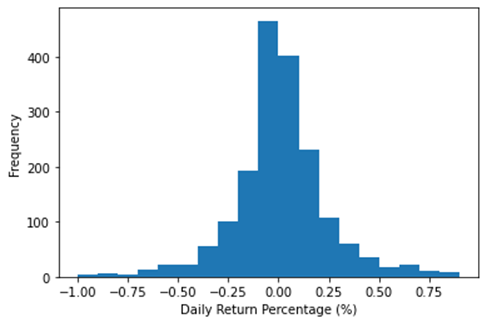
Figure 2: Original Strategy – Profit Changes with Tim.

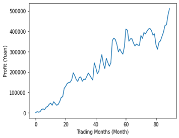
Figure 3: Original Strategy – Frequency of Daily Return Percentage.

The first two illustrate the continuous growth of our portfolio's net worth and profit over the years, albeit with fluctuations. Figure 3 displays the frequency distribution of the portfolio's daily return percentage, centered around 0.

3.2. Summary Statistics

3.2.1. Analysis

The strategy demonstrates a moderate level of return and volatility, with a 75% VaR of 0.09% and a maximum drawdown of 5%, which are considered acceptable. However, Table 6 indicates that the leptokurtic nature and negative skewness of the distribution highlight the potential for extreme losses. Additionally, the strategy exhibits a very low correlation with the market.

3.2.2. Data Check

The following checks were performed:

1. Verification of NaN or trivial values in high/low/settlement prices: It was observed that the settlement prices for each contract on a daily basis are available and non-trivial. Although some high/low prices were missing, they were substituted with the settlement price. The high/low prices are crucial for calculating the typical cost of each day.

2. Volume check on the signal generation day: Transactions are executed only if the notional volume on that date exceeds 50,000,000.

3. Remaining days until contract expiration: Only contracts with at least one month left for trading are considered. Positions associated with contracts having less than one month until expiration are mandatorily closed.

4. Adequacy of the security fund: Ensuring that the security fund is sufficient for trading.

5. Identification of extreme losses or gains in transactions.

6. Unit tests: Various tests are conducted, such as verifying if profits are calculated accurately, confirming correct results for randomly selected transactions, and validating that costs are negative.

3.3. Differences from Expectation

Table 7: Original Strategy – Differences from Expected Portfolio Performances.

The performance of our in-sample backtesting did not meet our expectations. The achieved annualized return and volatility are approximately one-third of the expected values, resulting in a lower Sharpe ratio of 0.27 compared to the expected 0.5.

4. Refinement

4.1. Refinement 1: Replacing Standard Deviations with ATR

In this refinement, we will replace standard deviations with ATR (Average True Range) in the signal generation and portfolio construction sections. ATR is calculated using the following formulas:

\( ATR=MA(TR, N) \)

\( {TR_{t}}= Max({High_{t}}-{Low_{t}}, |{High_{t}}-{Close_{t-1}}|, |{Close_{t-1}}-{Low_{t}}|) \)

The signal is then determined based on the difference between the current price and the moving average:

\( Signals=\frac{P-MA[TP, 20]}{2×ATR[TR, 20]} \)

Where:

MA = Moving average

\( TP(Typical Price)=\frac{High+Low+Close}{3} \)

Next, the unit size of each position is determined based on the calculated signals:

\( {Position Size_{i}}=c×1\%×Signal \)

To avoid overinvestment, the position size is limited to a maximum of 3% of the capital. The trading rules will remain unchanged.

Results

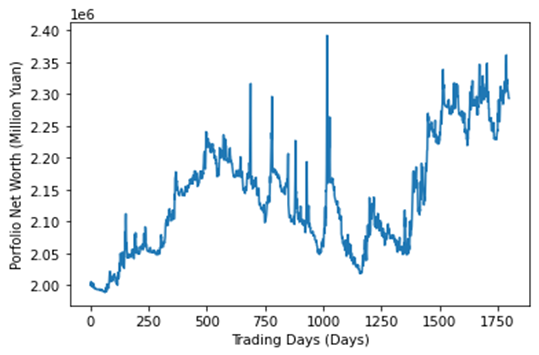
Figure 4: Refinement 1 – Portfolio Net Worth Changes with Time.

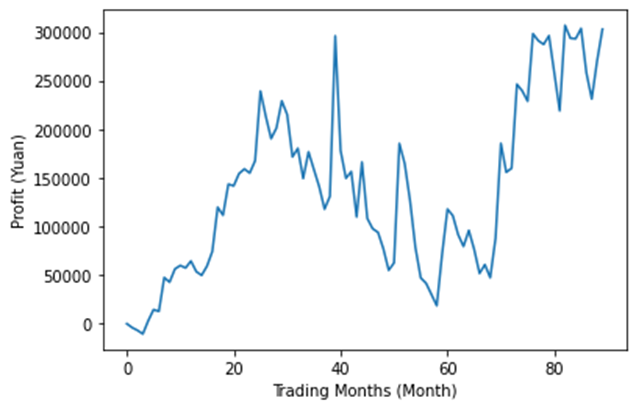
Figure 5: Refinement 1 – Profit Changes with Time.

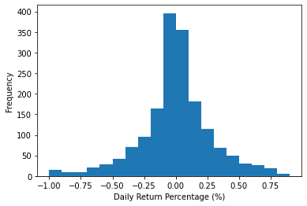
Figure 6: Refinement 1 – Frequency of Daily Return Percentage.

Statistics

Table 8: Refinement 1 – Statistics for Data Range from 2012/9 to 2020/2.

The results in Table 8 indicate that replacing standard deviations with ATR alone is not ideal. The return is lower, while risks are higher. Almost every metric per-formed worse, with increased general risk as the maximum drawdown nearly tripled and returns became highly concentrated. The current ATR signal formulas are not efficient enough. Therefore, we will not use ATR for our final selection. One possible modification for this method could be exploring different multipliers and shortening the period of ATR to better reflect recent fluctuations.

4.2. Refinement 2: Cross-Commodity Hedging

In this refinement, we introduce cross-commodity hedging. For each position in the portfolio, an opposite position is taken in the highest positively correlated commodity type. The hedging contract should have the same maturity and quantity as the original position.

\( Hedge Ratio = Correlation×\frac{{σ_{u}}}{{σ_{h}}} \)

\( Quantity of Hedging Contract ({Q_{h}}) = Hedge Ratio× {Q_{u}} \)

Where:

\( {σ_{u}} \) and \( {σ_{h}} \) are volatilities of unhedged contracts and hedging contracts.

\( {Q_{u}} \) and \( {Q_{h}} \) are quantities of unhedged contracts and hedging contracts.

Results

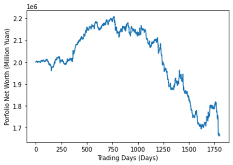
Figure 7: Refinement 2 – Portfolio Net Worth Changes with Time.

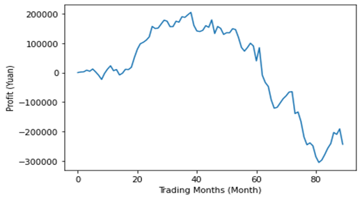
Figure 8: Refinement 2 – Profit Changes with Time.

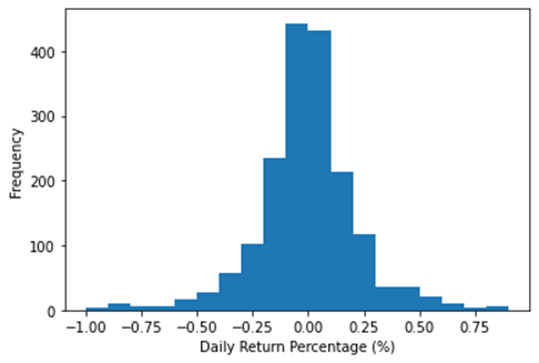
Figure 9: Refinement 2 – Frequency of Daily Return Percentage.

Statistics

Table 9: Refinement 2 – Statistics for Data Range from 2012/9 to 2020/2.

The addition of cross-commodity hedging slightly decreased volatility, but the return declined significantly, resulting in a negative Sharpe ratio. Sacrificing substantial returns for only a slight reduction in risk is not justified. The return is lower even when the win rate is 10% higher because frequent hedging transactions led to increased transaction costs while the average profit remained the same.

5. Out-Of-Sample Results & Trading Recommendations

5.1. Final Selection

After conducting multiple backtests, we have concluded that none of the individual refinements or their combinations improved our strategy. Therefore, we have decided to stick with our original strategy as it continues to yield the best results.

5.2. Out of Sample Backtest

Results

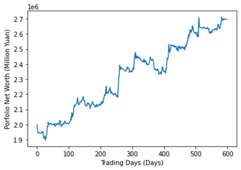
Figure 10: Out of Sample Backtest – Portfolio Net Worth Changes with Time.

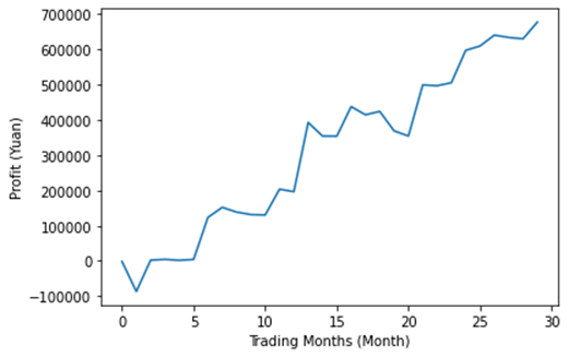
Figure 11: Out of Sample Backtest – Profit Changes with Time.

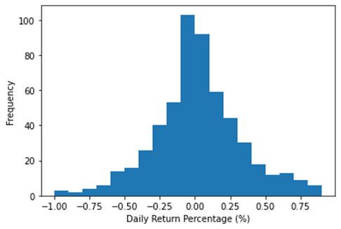
Figure 12: Out of Sample Backtest – Frequency of Daily Return Percentage.

Statistics

Table 10: Out of Sample Backtest – Statistics for Data Range from 2012/9 to 2020/2

The out-of-sample backtest shows a significantly higher return and Sharpe ratio compared to the in-sample test, while maintaining the overall risk at the same level. This indicates that the current volatile market conditions strongly favor our strategy.

5.3. Additional Considerations

Operations

Implementing this strategy does not pose challenges in terms of obtaining public transaction information. However, foreign investors may face difficulties trading in the Chinese futures market due to China's cautious approach towards foreign participation and the presence of trading restrictions. Nonetheless, China has made efforts to improve the efficiency of its securities markets, allowing qualified foreign capital to invest in various types of futures in the Chinese commodity market. Therefore, the findings of this study have important implications for the development of China's commodity markets. Gradual relaxation of foreign portfolio investment restrictions can contribute to improving the efficiency of commodity markets. It should be noted that our strategy, although relatively simple, may not perform as well in an efficient market, and the resulting Sharpe ratio may be lower than our current results. Furthermore, the strategy minimizes subjective errors as it relies on pre-set trading rules, and the risk is limited through the use of stop-loss conditions. However, false signals remain a potential challenge.

Correlation

The strategy, along with its refined versions, exhibits a low correlation with the market. This characteristic serves as a cushion during periods of high market volatility.

Future

This range breakout strategy based on the commodity futures is complex and requires expertise. However, given the similarity in trading rules, this type of strategy could become popular among traders. Historical data indicates that simi-lar range breakout strategies have not shown a significant decline in returns over the past 30 years. Considering the significant trading volume of China's commodity futures market and the growth of derivatives trading in the Asia-Pacific region, the capacity of this strategy can be further enhanced. Although the volatility characteristics of commodity markets make them particularly suitable for technical momentum strategies, this approach can also be applied to other asset classes and markets. [6]

Environment

Range breakout trading benefits from the comprehensive information and tools provided by most trading platforms. It is relatively straightforward to identify breakouts and access indicators that confirm price trends. Additionally, investors are attracted to the potential for quick payoffs when conditions align. The strategy allows for limited exposure to adverse market movements, ensuring that re-wards can be realized without enduring significant losses if the trend favors the trader.

5.4. Trading Recommendation

Based on the out-of-sample data, which yielded a much better return of 13.4572% compared to the in-sample data, and a decent Sharpe ratio of 1.34, we recommend implementing the strategy in the Chinese commodity market. The strategy has shown favorable performance, particularly in recent years when the market has been more volatile. However, it is important to note that performance may vary under different market conditions. Specifically, the strategy is expected to excel in market conditions where significant price trends in a specific commodity category have formed [7].

When trading commodity range breakouts, there are certain factors to consider:

1. Liquidity risk: It is advisable to avoid trading low-volume contracts and to liquidate positions early to mitigate the risk of a squeeze in near-month contracts.

2. Maximum position limit: Institutional investors with significant assets under management should be mindful of the maximum position limit, as it may pose challenges.

6. Conclusion

In conclusion, the original trading strategy exhibited average return and volatility, accompanied by an acceptable 75% VaR and maximum drawdown. However, the strategy displayed leptokurtic and negative skewness characteristics, indicating the potential for extreme losses. Moreover, the strategy demonstrated a very low correlation with the market. After thorough data checks and unit tests, the in-sample backtesting results did not meet expectations, prompting the introduction of refinements. Refinement 1, which involved replacing standard deviations with ATR, did not yield ideal results. Refinement 2 proposed cross-commodity hedging to enhance portfolio performance. Further modifications could be explored for the ATR method, and additional research could be conducted to identify the optimal hedging commodity. Overall, this study emphasizes the significance of data analysis, testing, and refinement in the development of a successful trading strategy.

Acknowledgements

Ruihan Deng and Jiayi Wang contributed equally to this work and should be considered co-first authors.

References

[1]. Ming-Ming, L. and Siok-Hwa, L. (2006) The Profitability of the Simple Moving Averages and Trading Range Breakout in the Asian Stock Markets. Journal of Asian Economics 17 (1): 144–70. https://doi.org/10.1016/j.asieco.2005.12.001.
[2]. Kung, J. (2009) Predictability of Technical Trading Rules: Evidence from the Taiwan Stock Market. Review of Applied Economics 5 (1-2). https://dotnetrest.lincoln.ac.nz/O365flowClient/cache/sites/www-content/Lincoln%20WWW/Documents/Faculties/COMMERCE/Review-of-Applied-Economics/Documentation-2008-2010/4-James%20J%20kung.pdf.
[3]. Gerritsen, D. F., Bouri, E., Ramezanifar, E., and Roubaud, D. (2019) The Profitability of Technical Trading Rules in the Bitcoin Market. Finance Research Letters, August. https://doi.org/10.1016/j.frl.2019.08.011.
[4]. Yu, H.,Nartea, G. V., Gan, C., and Yao, L. J. (2013) Predictive Ability and Profitability of Simple Technical Trading Rules: Recent Evidence from Southeast Asian Stock Markets. International Review of Economics & Finance 25 (January): 356–71. https://doi.org/10.1016/j.iref.2012.07.016.
[5]. PAUNA, C. (2019) Additional Limit Conditions for Breakout Trading Strategies. Informatica Economica 23 (2/2019): 25–33. https://doi.org/10.12948/issn14531305/23.2.2019.03.
[6]. Chevallier, J., and Ielpo F. (2014) ‘Time Series Momentum’ in Commodity Markets. Managerial Finance 40 (7): 662–80. https://doi.org/10.1108/mf-11-2013-0322.
[7]. Bessembinder, H., and Chan, K. (1998) Market Efficiency and the Returns to Technical Analysis. Financial Management 27 (2): 5. https://doi.org/10.2307/3666289.
Cite this article
Deng,R.;Wang,J.;Dong,H.;Lo,W.;Dong,H. (2023). The Implementation and Refinement of Range Breakout Strategy in Chinese Commodity Market. Advances in Economics, Management and Political Sciences,18,27-45.
Data availability
The datasets used and/or analyzed during the current study will be available from the authors upon reasonable request.
Disclaimer/Publisher's Note
The statements, opinions and data contained in all publications are solely those of the individual author(s) and contributor(s) and not of EWA Publishing and/or the editor(s). EWA Publishing and/or the editor(s) disclaim responsibility for any injury to people or property resulting from any ideas, methods, instructions or products referred to in the content.
About volume
Volume title: Proceedings of the 2023 International Conference on Management Research and Economic Development
© 2024 by the author(s). Licensee EWA Publishing, Oxford, UK. This article is an open access article distributed under the terms and
conditions of the Creative Commons Attribution (CC BY) license. Authors who
publish this series agree to the following terms:
1. Authors retain copyright and grant the series right of first publication with the work simultaneously licensed under a Creative Commons
Attribution License that allows others to share the work with an acknowledgment of the work's authorship and initial publication in this
series.
2. Authors are able to enter into separate, additional contractual arrangements for the non-exclusive distribution of the series's published
version of the work (e.g., post it to an institutional repository or publish it in a book), with an acknowledgment of its initial
publication in this series.
3. Authors are permitted and encouraged to post their work online (e.g., in institutional repositories or on their website) prior to and
during the submission process, as it can lead to productive exchanges, as well as earlier and greater citation of published work (See
Open access policy for details).