1. Introduction

The 2023 global growth, estimated mainly by the GDP considered as a significant indicator, is predicted to decline to 2.9 percent in 2023 but up to 3.1percent in 2024, is 0.2 percent higher than the October 2022 World economic outlook’s forecast but lower than the historical average of 3.8 percent. Economic activities are interfered dramatically by rising interest rates and the Russia to Ukraine military conflict [1]. Central banks facing stubbornly high inflation have taken actions such as the constantly tight currency policy to avoid entrenched inflationary pressures [2]. The impact of the net cumulative GDP gap caused by conflicts remains negative for most relevant countries [3]. production is disrupted by conflicts, and output is affected negative immediately [4]. Worldwide capital market has been impacted drastically. Portfolio optimization strategies is considered by investors to adjust risks amid increase expected returns in this burdensome period.

Based on a given risk level, the maximum portfolio returns are acquired by choosing the best asset allocations are aimed by the optimization [5]. Nevertheless, Kahneman & Tversky have found that more risks are undertaken willingly by people to choose loss avoidances, instead of realizing rewards [6]. Investors are risk-averse confronting returns, nevertheless, investors become risk seeking confronting losses. Quantified expected return-to-risk trade-off adjustments is necessary. Used in an informed tendency, quantified measures are veridical, advantages of quantifications are interpreted vividly by Charney: public and private scrutiny learn quantitative method firmly and share efficiently. Possessing the characteristic reliability, quantitative measures are formal, couldn’t be restricted by geographic and temporal distance, don’t take notice of experience and background, could ignore a shared natural language absence [7]. The returns from the financial market (excessing the risk-free rate) have aroused transactional managers and investors’ increased attentions, are divided by the standard deviation, a measure known as the sharpe ratio is derived [8]. According to MPT, the maximum sharpe ratio portfolio locates on the efficient frontier of mean-variance [9]. And after obtaining the optimal portfolio, some certain indicators are needed to evaluate the performance of the portfolio [10].

The shortage of global portfolios constructed by indexes research is existent presently. The major research orientation is the study refers to industrial portfolios. Yehuda and David analyzed a portfolio model, by which the property-liability insurance industry’s insurance and investment portfolios were simultaneously optimized. The conclusion is that the company’s investment policy isn’t necessary to implement more conservative when the risk of insurance portfolio is increased [11]. Noureddine and Amin adopts a fuzzy interval goal programming approach to study the sustainable and renewable energy portfolio optimizations, which is a proposed methodology, capably assisting the DMs in the RE optimized portfolio ascertainment in imprecise environments and under a highly uncertain level [12]. Wu and other colleagues studied the renewable energy project (REP) portfolio efficiency optimizations with the support of a fuzzy multi-criteria decision-making (MCDM) framework [13]. HOU and DAVID studied the CRSP monthly returns file and the COMPUSTAT industrial annual file’s intersections contained all NYSE-, AMEX-, and NASDAQ-listed securities with share condes 10 or 11 during July 1963 to December 2001, drew the conclusion that the risk of highly concentrated industrial companies is down, because enterprises participate in less innovations, therefore, less expected returns are obtained [14].

This paper targets to make an analysis about portfolio optimization efficiency, portfolio management strategies references were offered to individual investors during this thriving period. 5 global indexes constructures the portfolios. Scipy optimization stimulation was used to calculate numerous portfolios, the maximum sharpe ratio and the minimum risk portfolios’ assets weights were gained. The cumulative returns comparisons of 1/N, 2 risk-based optimizations portfolios were observed visually, therefore, the conclusion was drawn. The results presented that the maximum sharpe ratio overcomes 1/N and the minimum volatility portfolios. A stability exam is implemented to prove valid rational quality of the methodologies and outcomes.

This article is organized as follows, representative indexes selected, and data used in the research were illustrated in section 2. Methodologies of constructing the efficient frontier and point out the maximum sharpe ratio and the minimum variance portfolios were described in section 3. Interprets results and check consequences of stability are interpreted in section 4. Section 5 draws the conclusion at the end.

2. Data

This paper chooses major 5 influential stocks indexes based on the financial market reflected fluctuated ratios of each nation’s stock market from wind financial terminal. The indexes are as follow: DJIA, Nikkei 225, FTSE100, SSE Composite Index, CAC40. Closing prices from February 24th, 2021, to February 24th, 2023, are gathered and divided into training set and test set. In order to plot the efficient frontier, the training set are used to calculate average returns and covariance matrices. The test set is used to evaluate performances of the chosen asset allocations via comparisons of the cumulative returns computed with maximum sharpe ratio model, minimum risk model and 1/N portfolio model ’s weights. Fundamentals of 5 selected assets are listed in Table1, Table2, Table 3, Fig. 1, respectively. In the duration, CAC40 achieved the highest average rate of return, FTSE100's smallest standard deviation shows the minimum risk. Fig. 1 reveals FTSE100 has the highest cumulative return of 7.622%, the cumulative return of SSE Composite Index decreased and reached -9.816% on the contrast finally.

Table 1: Chosen assets.

Table 2: Descriptions of the selected data.

Table 3: Covariance matrix.

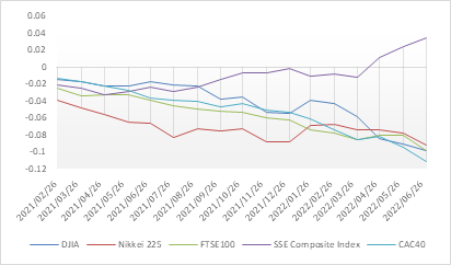
Figure 1: Cumulative returns.

3. Methods

The mean variance model is applied usefully when comprehensively thinking about portfolio expected returns and risks. The function of portfolio returns and variances.

\( {r_{ρ}}=\sum _{i}{w_{i}}{r_{i}} \) (1)

Where portfolio \( {i^{th}} \) component weight and expected return are \( {w_{i}} \) and \( {r_{i}} \) respectively. The details for deviation are shown below.

\( {r_{ρ1}}={w_{1}}\bar{{r_{1}}}+{w_{2}}\bar{{r_{2}}}+{w_{3}}\bar{{r_{3}}}+{w_{4}}\bar{{r_{4}}}+{w_{5}}\bar{{r_{5}}} \) (2)

\( σ_{ρ}^{2}=\sum _{i}r_{i}^{2}w_{i}^{2}+\sum _{i}\sum _{j}{σ_{i}}{σ_{j}}{w_{i}}{w_{j}}{ρ_{ij}} \) (3)

\( {σ_{ij=\sum _{m=1}^{n}{ρ_{m}}}}({i_{m}}-\bar{i})({j_{m}}-\bar{j}) \) (4)

Where \( {σ_{i}} \) is \( i \) index's standard deviation, covariance. Three strategic portfolios are considered in this article and could be observed on the efficient frontier: the maximum sharpe ratio portfolio, the minimum variance portfolio and 1/N portfolio. 1/N portfolio is used commonly because investors prefer to distribute currency evenly and invest into several assets. The habitual investment method 1/N portfolio is taken into consideration. The sharpe ratio is used to quantify the adjusted risk comprehensively, the following is the function.

\( Sharpe ratio=\frac{{r_{ρ}}-{r_{f}}}{{σ_{ρ}}} \) (5)

Where \( {r_{ρ}} \) is the expected return of the portfolio, \( {r_{f}} \) is the free risk rate (namely 10 years American national bond return rate) and \( {σ_{ρ}} \) is the standard deviation. Portfolio with higher sharpe ratio will acquire more expected returns if its volatility is same. Risk adjustment performance of the maximum sharpe ratio surpasses other portfolios.

4. Empirical Results

10,000 times random portfolio weights calculations were performed with scipy optimization functions, presentations of gathered scatters are as follow (Fig. 2), upward edge curve is the efficient frontier. The scatter represents each portfolio's individual expected return ratio and risk, recession curve (sharpe ratios are minus) means the same undertaken risk with lower expected inefficient return (investors pursue the largest margins).

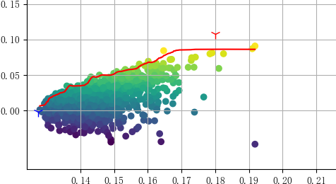
Figure 2: Efficient frontier.

The minimum variance and the maximum sharpe ratio portfolios were found on the efficient frontier, two premium portfolios are labeled on Fig. 2, the minimum risk portfolio locates on the left limitation of the efficient frontier, indexes weights are: DJIA, 0.3425; Nik.kei, 0.0929; FTSE100, 0.2136; SEE, 0.3511; CAC40, 1.7998E-17. The maximum sharpe ratios portfolio weights are: DJIA, 2.8549E-16; Nik.kei, 0.0000; FTSE100, 1.0000; SEE, 3.8246E-17; CAC40, 0.0000 (Table4 presents). The minimum risk portfolio's deviation is 0.1273, the maximum sharpe ratio portfolio's slope is 0.5691 (details on Table5). For the minimum risk portfolio, SSE Composite Index accounts for 35.11% while FTSE100 proportion possesses approximately 100% in the maximum sharpe ratio portfolio. CAC40 indexes possessions in both portfolios are slightly tiny insignificantly (See Table 4 and Table 5).

Table 4: Weight of each asset in 2 optimized portfolios.

Table 5: Characteristics of 2 optimal portfolios.

Using test sets from July 20th, 2022, to February 24th, 2023, with two obtained asset allocations’ weights, the daily portfolio return ratios could be calculated, furthermore, the cumulative returns were gained. The cumulative return of the maximum sharpe ratio portfolio is 4.8144%, that of the minimum risk portfolio is 0.1712% and 1.1942% in 1/N portfolio, the maximum sharpe ratio portfolio and 1/N portfolio surpass the minimum risk portfolio under most circumstances. The maximum sharpe ratio portfolio performs optimally, compared with the minimum volatility portfolio and 1/N portfolio (See Table 6).

Table 6: Cumulative returns comparisons

The method of stability test would be applied to check the results’ certainty. Firstly, eliminate CAC40 from the portfolio components because of slightly tiny percentage. Secondly, 10000 scipy optimization simulations operate again and compute the new cumulative return. The remaining indexes weights for 2 optimal portfolios are listed in Table 7, observation: FTSE100 takes up approximately 100% in the maximum sharpe ratio portfolio, SSE Composite Index takes up 35.32% in the minimum volatility portfolio, indicate that the largest proportion assets in 2 portfolios keep the same. Finally, compute and compare 3 portfolio cumulative returns (See Table 8), those're similar to the previous results where the maximum sharpe ratio portfolio has the highest cumulative return. Thus, the methods and outcomes are effective and stable.

Table 7: 4 remaining indexes' weights in 2 optimized portfolios.

Table 8: Comparisons.

5. Conclusion

Three merit portfolios (the maximum sharpe ratio, the minimum volatility and 1/N) constructed by 5 representative indexes were investigated in this article in general. Acquired data from wind finance, portfolios’ cumulative returns during the sustainable stiff period were obtained. Calculated randomly ten thousand portfolios by scipy optimization, each portfolio’s expected return correspondence volatility was computed consequently. By gathering the portfolios scatters (represent expected returns against risks), the visualized data was presented, the efficient frontier curve could be plotted. Two optimal portfolios’ assets allocations were gained. 1/N portfolio was calculated additionally, equal assets allocations, haven access to the test set, the cumulative portfolio returns were worked out.

Via comparisons among three portfolios, it could be observed that the maximum sharpe ratio portfolio performs optimal with obtaining the highest return, surpassed 1/N and the minimum volatility portfolios. FTSE100 takes up approximately 100% in the maximum sharpe ratio portfolio before and after the stability test, showing that investors hold a common perspective pursuing the largest benefit, could put more currency weights on the FTSE100, a remarkable asset.

However, several deficiencies also exist in this study. For example, constant correlation is considered, actually, dynamic correlation rather than constant correlation is more suitable for financial assets, thus, this investigation seems limited. Considering the dynamic correlation estimated by multi-GARCH models deserves the in-depth focus.

References

[1]. World Economic Outlook Update projects, https://www.imf.org/en/Publications/WEO/Issues/2023/01/31/world-economic-outlook-update-january-2023, last accessed 2023/1/30.
[2]. Volatile Markets Signal Rising Financial Stability Risks, https://www.imf.org/en/Blogs/Articles/2022/10/11/interest-rate-increases-volatile-markets-signal-rising-financial-stability-risks, last accessed 2022/10/11.
[3]. De Groot, O. J., Bozzoli, C., Alamir, A., Brück, T.: The global economic burden of violent conflict. Journal of Peace Research 59(2), 259-276 (2022).
[4]. Blomberg, S. B., Hess, G. D., Orphanides, A.: The macroeconomic consequences of terrorism. Journal of monetary economics 51(5), 1007-1032 (2004).
[5]. Zhang, Z., Zohren, S., Roberts, S.: Deep learning for portfolio optimization. The Journal of Financial Data Science 2(4), 8-20 (2020).
[6]. Berkelaar, A. B., Kouwenberg, R., Post, T.: Optimal portfolio choice under loss aversion. Review of Economics and Statistics 86(4), 973-987 (2004).
[7]. Elliot, N., Briller, V., Joshi, K.: Portfolio assessment: Quantification and community. Journal of writing assessment 3(1), (2007).
[8]. Sharpe, W. F.: Mutual fund performance. The Journal of business 39(1), 119-138 (1966).
[9]. Kourtis, A.: The Sharpe ratio of estimated efficient portfolios. Finance Research Letters 17, 72-78 (2016).
[10]. FAIZ, M.: ANALISIS PERBANDINGAN KINERJA SAHAM SYARIAH DAN SAHAM KONVENSIONAL PADA SEKTOR MANUFAKTUR DI MASA PANDEMI COVID-19. Universitas Gadjah Mada, Thesis for Doctoral degree (2022).
[11]. Kahane, Y., Nye, D.: A Portfolio Approach to the Property-Liability Insurance Industry. The Journal of Risk and Insurance 42(4), 579–598 (1975).
[12]. Kouaissah, N., Hocine, A.: Optimizing sustainable and renewable energy portfolios using a fuzzy interval goal programming approach. Computers & Industrial Engineering 144, 106448 (2020).
[13]. Wu, Y., Xu, C., Ke, Y., Tao, Y., Li, X.: Portfolio optimization of renewable energy projects under type-2 fuzzy environment with sustainability perspective. Computers & Industrial Engineering 133, 69-82 (2019).
[14]. Hou, K., Robinson, D. T.: Industry concentration and average stock returns. The journal of finance 61(4), 1927-1956 (2006).
Cite this article
Luo,N. (2023). Optimized Portfolio Structured by 5 Stock Indexes. Advances in Economics, Management and Political Sciences,24,13-19.
Data availability
The datasets used and/or analyzed during the current study will be available from the authors upon reasonable request.
Disclaimer/Publisher's Note
The statements, opinions and data contained in all publications are solely those of the individual author(s) and contributor(s) and not of EWA Publishing and/or the editor(s). EWA Publishing and/or the editor(s) disclaim responsibility for any injury to people or property resulting from any ideas, methods, instructions or products referred to in the content.
About volume
Volume title: Proceedings of the 2023 International Conference on Management Research and Economic Development
© 2024 by the author(s). Licensee EWA Publishing, Oxford, UK. This article is an open access article distributed under the terms and
conditions of the Creative Commons Attribution (CC BY) license. Authors who
publish this series agree to the following terms:
1. Authors retain copyright and grant the series right of first publication with the work simultaneously licensed under a Creative Commons
Attribution License that allows others to share the work with an acknowledgment of the work's authorship and initial publication in this
series.
2. Authors are able to enter into separate, additional contractual arrangements for the non-exclusive distribution of the series's published
version of the work (e.g., post it to an institutional repository or publish it in a book), with an acknowledgment of its initial
publication in this series.
3. Authors are permitted and encouraged to post their work online (e.g., in institutional repositories or on their website) prior to and
during the submission process, as it can lead to productive exchanges, as well as earlier and greater citation of published work (See
Open access policy for details).