1 Introduction

The coronavirus pandemic has spread swiftly after the first COVID-19 case was discovered in China in December 2019. Even though China has prevented the pandemic from worsening, the global pandemic will undoubtedly have an impact on the world economy, including China, in the beginning of 2020. The pandemic has now widely dispersed overseas. Due to actions made by governments of various countries to close the country, states, and cities, several sectors around the world have been badly damaged by the inability of production factors to freely flow in the market. The global industrial chain is also broken, many companies are unable to carry out normal production, and demand on the global market is declining. In addition, many countries, Several nations, including the US, South Korea, and the Philippines, witnessed stock market circuit breakers when the global stock market fell. Even the US stock exchange has four circuit breakers [1].

In February 2020, the World Health Organization declared a public health emergency. Around a month later, on March 11, 2020, epidemiologists from the World Health Organization classified COVID 19 as a global pandemic [2]. Between February 3, 2020, and June 17, 2022, 98,827,261,177 confirmed instances were reported globally, according to Our Data World. Furthermore, the global average is still increasing by about 150,000 cases every day. The Covid-19 pandemic has had an impact on more than 200 countries and has caused an unprecedented global health emergency [3].

The COVID-19 pandemic has disrupted the textile, apparel, and fashion manufacturing (TAFM) industry's supply chain in a variety of previously unheard-of ways over the past few months, as seen by people all around the world [4]. Due to travel restrictions and a shortage of raw materials, this outbreak has a global impact because of how interwoven the world's textile markets are.

In the expert introduction, it is further discussed how the COVID-19 pandemic, which resulted in more than 88 million infections and more than 1.8 million fatalities, has had negative effects on the environment, travel, education, clinical research, human and animal health globally, as well as on human civilization, agriculture, and global socioeconomics. Although vaccination applications have just begun, it is yet unknown how efficient, durable, affordable, prone to cause anaphylaxis, and likely to result in reinfection these vaccines will be due to new variations and mutations. When compared to living conditions prior to the pandemic, the middle income can survive, but there is still a substantial imbalance that adversely impacts economically disadvantaged families, marginalized communities in Purba Bardhaman, the elderly, and street urchins, and creatures [6].

An unprecedented drop in worldwide activity has been brought about by the COVID-19 pandemic. In industrialized and emerging economies, the pandemic's growing effects prompted strict lockdowns and significant disruptions of economic activity at an exceptional rate and scale [7]. For instance, economic disruption caused the global GDP to fall by more than 4.9 percent in the second quarter of 2020. Traded goods and services plummeted more than they did during the world financial crisis of 2007–2008. The second quarter of 2020 saw a 3.5 percent fall in global commerce due to weak demand and supply. The COVID-19 lockout interrupted worldwide supply chains, which hampered demand all around the world [8]. Due to the large income loss and low consumer confidence, there was a considerable fall in the consumption of goods and services. Due to concerns about the COVID outbreak, consumers were hesitant to use products and services [9]. Due to a sharp fall in demand, disruptions in the supply, and unclear future revenue, businesses were forced to reduce their investment. Following 130 million full-time mass layoffs in the first quarter of 2020, there were about 300 million comprehensive job losses globally in the second quarter. Disinflation and fuel prices are the results of the general fall in demand.

This article examines how manufacturing and biopharmaceutical index prices have changed because of the pandemic using the timeline of Covid-19's outbreak and spread to study the regulations and practices that have contributed to these changes.

The remainder of this essay is structured as follows: part 2 is research design, which includes data sources, unit root test, and model specification; Part 3 reports empirical results, including VAR and ARMA-GARCH estimation results; Part 4 is discussion and part 5 is the conclusion.

2 Research Design

2.1 Data Sources

The manufacturing index, biopharmaceutical industry index, and other financial data used in this article were taken from the Yahoo Finance website. Every day starting on February 3, 2020, with Covid-19 cases present all across the world, adjusted closing prices are chosen. The charity Global Change Data Lab in the UK maintains the "Our World in Data" website, which offers details on recently confirmed instances across the globe including in China. The high quality of the data is demonstrated by the fact that it is used in hundreds of articles and reports each year. All of the data used in the analysis of the remaining portions of the paper are logarithmic, therefore information about stock prices refers to the logarithm of the price, and information about recently confirmed cases refers to the logarithm of instances, etc.

2.2 ADF-Test

It is necessary to test each variable's stationarity before building models.

The time series variable's nonstationarity is the unit root test's null hypothesis.

\( {y_{t}}=α+p{y_{t-1}}+\sum _{i=1}^{p-1}{ζ_{i}}Δ{y_{t-i}}+ε\ \ \ (1) \)

The null hypothesis \( {H_{0}}:p=1 \) and the alternative hypothesis \( {H_{1}}=p \lt 1 \) .

Decision rule: reject the null hypothesis when ADF test= \( \frac{\hat{p}-1}{SD} \) is bigger than the critical value.

While the stock price has a non-stationary distribution and a p-value above 0.05, Table 1 demonstrates that the return rate, newly confirmed occurrences in China, and the global average all seem to have motionless distributions and p-values below 0.05.

Table 1. ADF test.

2.3 Model Specification: VAR

To examine the dynamic influence of returns on manufacturing and pharmaceutical indexes according to COVID-19, this part builds a VAR model. To ensure that the predictions are mutually compatible, the variables are combined and predicted as a single system.

Model settings are as follows:

\( {y_{t}}=(\begin{matrix}{β_{10}} \\ {β_{20}} \\ \end{matrix})+(\begin{matrix}{β_{11}} & {γ_{11}} \\ {β_{21}} & {γ_{21}} \\ \end{matrix}){y_{t-1}}+⋯+\begin{matrix}{β_{1p}} & {γ_{1p}} \\ {β_{2p}} & {γ_{2p}} \\ \end{matrix}{y_{t-p}}{ε_{t}}\ \ \ (2) \)

In (2), \( {y_{t}}=\begin{cases}{y_{1t}},{y_{2t}}\rbrace \end{cases} \) is a vector of two-time series, 𝜀𝑡 is the disturbance term and 𝑝 refers to the time lag this part take.

The impact of a single unit disturbance on how other variables will evolve over time is examined through the impulse response function.

The model looks like this:

\( \frac{{∂_{{y_{t+s}}}}}{{∂_{{ε_{t}}}}}=φ\ \ \ (3) \)

This equation determines how much the disturbance term t of the variable at the t-th period changes the value of the variable at the (t+s)-th period, \( {y_{t+s}} \) , while other variables and disturbance terms in other periods do not change.

2.4 ARMA-GARCH Model Specifications

This part now build the ARMA-GARCH model, which will simultaneously predict the rate of return and volatility of the manufacturing index and biopharmaceutical industry index. As exogenous variables, utilize the most recent confirmed cases in China and globally, respectively.

Thus, this part can assess the relationship between the outbreak status and the yield and stock volatility.

This is how the model ARMA (p, q) is configured:

\( {x_{t}}={ϕ_{0}}+{ϕ_{1}}{x_{t-1}}+⋯+{ϕ_{p}}+{x_{t-p}}+{ε_{t}}+{θ_{1}}{ε_{t-1}}+⋯+{θ_{q}}{ε_{t-q}}\ \ \ (4) \)

This is how the model GARCH (p, q) is configured:

\( {σ_{t}}={α_{0}}+{α_{1}}{{ε_{t-1}}^{2}}+⋯+{α_{q}}{{ε_{t-q}}^{2}}+{γ_{1}}{{σ_{t-1}}^{2}}+⋯+{γ_{p}}{{σ_{t-p}}^{2}}\ \ \ (5) \)

The word \( {α_{1}}ε_{t-1}^{2}+⋯+{α_{q}}ε_{t-q}^{2} \) is ARCH portion in (5). The disturbance term's conditional variance is represented by the subscript \( {ε_{t}} \) , which denotes that variance varies over time. The square of the disturbance term in the previous p periods determines how \( σ_{t}^{2} \) behaves.

The ARCH model serves as the foundation for the GARCH model, which also includes the autoregression of \( σ_{t}^{2} \) . The word \( {γ_{1}}σ_{t-1}^{2}+⋯+{γ_{p}}σ_{t-p}^{2} \) is a GARCH component in (4).

The GARCH model is made to have fewer parameters. By repeatedly iterating, this portion can reduce ARCH(p) to GARCH (1,1).

3 Research Design

3.1 VAR

The VAR identification methods are LR, FPE, AIC, HQIC, and SBIC. The method used in this paper is LR. In addition, for the consideration of stationarity, before establishing the VAR model, this part have to first judge whether each variable has stationarity. Only by performing OLS estimation on the VAR model composed of stationary variables can this part obtain consistently estimated parameters.

Determination of the maximum lag order k: LR

\( LR=-2(Log{L_{k}}-Log{L_{k+1}}), LR~x_{({N^{2}})}^{2}\ \ \ (6) \)

(1). When the LR statistic is less than the critical value, the lag order of the VAR model is considered to be moderate

(2). The lag order of the VAR model is deemed to be insufficiently high when the LR statistic exceeds the critical value, necessitating the addition of additional lag variables as explanatory variables.

(3). The asymptotic distribution of LR differs significantly from the finite sample distribution of LR when the sample size is insufficient relative to the number of calculated parameters.

Then, Stability conditions for VAR:

\( {X_{t}}=\sum _{i=1}^{p}{Π_{i}}{X_{t-i}}+{U_{t}}\ \ \ (7) \)

(1). The necessary and sufficient condition of the VAR model is that all eigenvalues of the coefficient matrix fall within the unit circle

(2). The conditions for judging the stationarity of the VAR model are essentially the same as the conditions for judging the stationarity of the AR model.

According to Table 2, the order of the VAR model is 12.

Table 2. VAR model identification.

This part have to first check the stationarity of the parameters before this part estimate them.

For this part to claim that this VAR system is stationary, all the roots of the characteristic equation \( |A-λI|=0 \) have to be located within the unit circle.

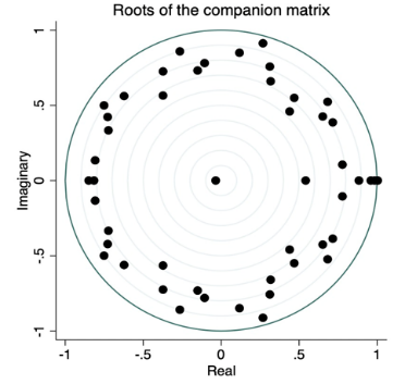Figure 1 shows the outcome. The VAR system is stationary because all of the black dots in Figure 3 are contained within the unit circle.

Fig 1. stationarity estimation using the characteristic equation's roots.

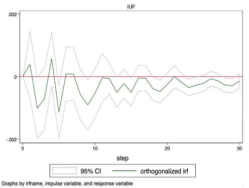
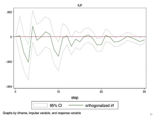
Humans will now design the impulse response diagram leveraging China or the international pandemic as the impulse variable and the stock return as the response variable. Figure 3 investigates the connection within China, whilst Figure 2 analyzes the relationship globally.

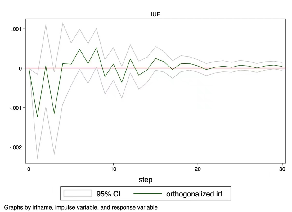
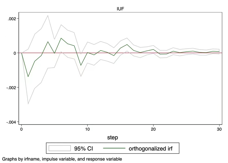
Figures 2 and 3 show contrary to common perception, the new crown pneumonia pandemic has not led to an increase in the profitability of the pharmaceutical industry.

From the perspective of the domestic pandemic, the current increase in the number of confirmed diagnoses in China and around the world will cause the pharmaceutical industry's yield to fluctuate in the future.

Although the size of the effect will diminish over time, the duration of the effect on the number of confirmed cases in China and the rest of the world is vary depending on when the shock occurred. The rate of return was only altered by the rise in confirmed diagnoses in China during the time t=0 for the first 15 or so periods, but the rate of return change brought on by the rise in confirmed diagnoses globally did not tend to zero out after 30 periods.

Accordingly, this study believes that the global pandemic has a greater impact on the pharmaceutical industry.

Combining the basic facts, it can be found that in the early stage of the new crown pneumonia pandemic, the profitability of the pharmaceutical industry increased rapidly, and then fell off a cliff in the later stage. In the long run, the new crown pneumonia is still a short-term positive, and the market reaction is excessive.

3.2 ARMA-GARCH

This part use the variable \( {X_{t}} \) to represent a time series, \( {x_{t}} \) represents the t-th point in the sequence, t=1,2,3,4...N, where N represents the length of the sequence \( {X_{t}} \)

The mean of the series:

\( μ=E({X_{t}})\ \ \ (8) \)

The variance of the series:

\( {σ^{2}}=D({X_{t}})=E({({X_{t}}-μ)^{2}})\ \ \ (9) \)

The standard deviation of the series: \( σ \)

For two different sequences \( {X_{t}} \) and \( {Y_{t}} \) of the same length, covariance can be used to characterize their correlation.

Covariance of series:

\( cov({X_{t}}, {Y_{t}})=E({(X_{t}}-{μ_{x}})({Y_{t}}-{μ_{y}}))\ \ \ (10) \)

The larger the covariance value \( cov({X_{t}}, {Y_{t}}) \) is, the stronger the correlation between the series \( {X_{t}} \) and \( {Y_{t}} \) is (positive correlation when greater than 0, negative correlation when less than 0). Similarly, for series \( {X_{t}} \) , this part calculate the corresponding series autocovariance according to the lag times k of the series.

The calculation formula of ACF is as below:

\( acf(k)={r_{k}}=\frac{{c_{k}}}{{c_{0}}}=\frac{N}{N-K}×\frac{\sum _{K+1}^{N}({x_{t}}-μ)({x_{t-k}}-μ)}{\sum _{T=1}^{N}({x_{t}}-μ)({x_{t}}-μ)}\ \ \ (11) \)

\( a\hat{c}f(k)={\hat{r}_{k}}=\frac{(N-k){c_{k}}}{N{c_{0}}}=\frac{\sum _{T=K+1}^{N}({x_{t}}-μ)({x_{t-k}}-μ)}{\sum _{t=1}^{N}({x_{t}}-μ)({x_{t}}-μ)}\ \ \ (12) \)

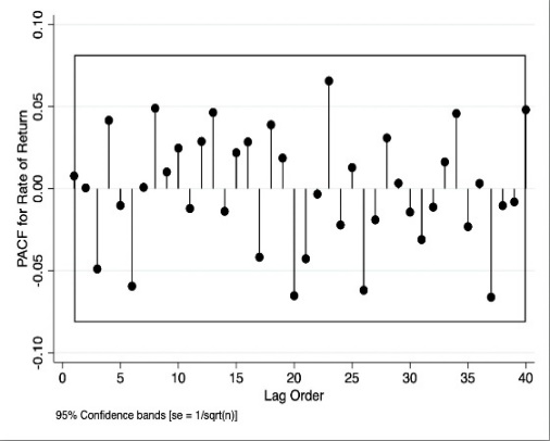
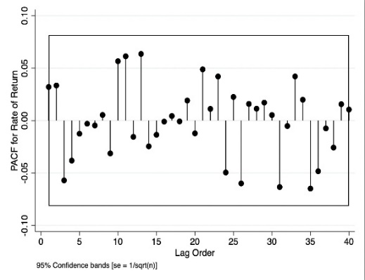
This section must first apply PACF to determine the AR model's order: The AR model is ordered using the ACF, which is a function of the PACF of a stationary time series.

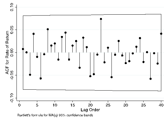
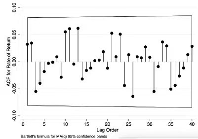
Now, this section has to use the ACF test to establish the MA model's order.

From the estimation result of the variance equation. Whether it is the pharmaceutical industry or the manufacturing industry, both the ARCH and GARCH terms are significant. It shows that the returns of these two industries have obvious conditional heteroscedasticity, which is suitable for GARCH modelling. Judging from the estimated results of exogenous variables, the number of confirmed diagnoses did not increase the volatility of the yields of the pharmaceutical industry and manufacturing industry.

As a result, this study's overall finding remains that the current crown pandemic has no overall influence on the pharmaceutical and manufacturing industries.

Table 3 ARMA-GARCH estimation results, variance equation.

4 Discussion

The measures that both industry indices should adopt to minimize potential losses from a similar situation in the future could be the subject of further study.

The findings of this study demonstrate that the public's restrictions on leaving the house and conducting business have led to significant short-term volatility in the manufacturing and biomedical sectors. This is in line with Jiaze Sun's earlier literature conclusions, which suggested that the pandemic will present significant development chances for the growth of manufacturing in China and possibly the entire world.

After COVID-19 subsides, the general trend in industrial output will revert to baseline levels. The importance of Chinese manufacturing in the global value chain will grow when the COVID-19 pandemic passes, however, manufacturers from the "Belt and Road" republics, the European Union, and the United States will diminish their involvement at meetings of the global value chain.

China will experience the highest rate of growth in the GVC's value-added exports in 2035, particularly in the export of complex GVC products, and imports will decline significantly. This suggests that the pandemic presents a significant chance for China to hasten its ascent to the top of the value chain.

The fact that China will continue to rely extensively on complicated GVC items imported from the US suggests that the US will continue to have some long-term influence over China's high-end manufacturing sector [10].

Although existing costs are solid due to evaporating revenue, the market is optimistic going forward. Investors don't need to worry too much, as the pandemic is about to pass and the stock market is trying to get back to where it was before the pandemic. For policymakers, looking to the future, everything can be implemented as normal, and the impact of the pandemic has been minimal. Likewise, for pandemics such as these, the impact on the world will only be in the early stage, compared to the early stage, the long-term impact will be negligible.

5 Conclusion

The pandemic has significantly affected the world economy. The returns of the manufacturing and biomedical indices were also severely impacted by the Covid-19 pandemic. In addition to providing additional proof of the pandemic's effects, this article focuses on the effect of Covid-19 on the returns and volatility of the industrial and biopharmaceutical indexes. This section found that Covid-19 had a minor long-term impact on stock returns, however, the pandemic had a short-term detrimental effect on manufacturing and biomedical index returns.

References

[1]. Li S, Yan Y, DATA-driven shock impact of COVID-19 on the market financial system, Science Direct, 1-3(2022).
[2]. World Health Organization. 2020. WHO coronavirus disease (COVID-19) dashboard, https://covid19.who.int/table, last accessed 2022/07/07.
[3]. Our World in Data. 2020. Statistics and Research: Coronavirus Pandemic (COVID-19), https://ourworldindata.org/coronavirus#growth-of-%20cases-how-long-did-it-take-for-the-number-of-%20confirmed-cases-to-double, last accessed 2022/07/07
[4]. Chakraborty, Samit, Biswas, Chandra Manik, Journal Supply Chain Management, Logistics and procurement, Henry Stewart Publications, (2020)
[5]. Subhas C Datta, Students Act as 21st Century Preventive-Pandemic-COVID-19 Model: Improved Advance-Clinical-Toxicology Biomedicine Green-Socio-Economy Science-Technology-Innovations, ISSN:2577-4328, 2-4(2021).
[6]. Patel Piyush, Gohil Piyush, Role of additive manufacturing in medical application COVID-19 scenario: India case study, 811-822, (2021)
[7]. Richard Baldwin, Beatrice Weder D Mauro, Mitigating the COVID Economic Crisis: Act Fast and Do Whatever It Takes, CERR Press, UK (2020)
[8]. C.T. Vidya, C.T. Prabheesh, Implications of COVID-19 Pandemic on the Global Trade Networks, Emerging Markets Finance and trade, 2408-2421(2020).
[9]. Martin S Eichenbaum, Rebelo Sergio, Trabandt Mathias, The Macroeconomics of Epidemics, 5149-5187(2021).
[10]. Sun J, Lee H, Yang J, Sustainability 2021, 13(22), The Impact of the COVID-19 Pandemic on the Global Value Chain of the Manufacturing Industry.
Cite this article
Yuan,Z. (2023). The Time-varying Impact of the Covid-19 Pandemic on Biopharmaceutical Industry and Manufacturing. Advances in Economics, Management and Political Sciences,4,538-547.
Data availability
The datasets used and/or analyzed during the current study will be available from the authors upon reasonable request.
Disclaimer/Publisher's Note
The statements, opinions and data contained in all publications are solely those of the individual author(s) and contributor(s) and not of EWA Publishing and/or the editor(s). EWA Publishing and/or the editor(s) disclaim responsibility for any injury to people or property resulting from any ideas, methods, instructions or products referred to in the content.
About volume
Volume title: Proceedings of the 6th International Conference on Economic Management and Green Development (ICEMGD 2022), Part Ⅱ
© 2024 by the author(s). Licensee EWA Publishing, Oxford, UK. This article is an open access article distributed under the terms and
conditions of the Creative Commons Attribution (CC BY) license. Authors who
publish this series agree to the following terms:
1. Authors retain copyright and grant the series right of first publication with the work simultaneously licensed under a Creative Commons
Attribution License that allows others to share the work with an acknowledgment of the work's authorship and initial publication in this
series.
2. Authors are able to enter into separate, additional contractual arrangements for the non-exclusive distribution of the series's published
version of the work (e.g., post it to an institutional repository or publish it in a book), with an acknowledgment of its initial
publication in this series.
3. Authors are permitted and encouraged to post their work online (e.g., in institutional repositories or on their website) prior to and
during the submission process, as it can lead to productive exchanges, as well as earlier and greater citation of published work (See
Open access policy for details).