1. Introduction

In the context of the current economic transformation from a stage of rapid growth to a stage of high-quality development, improving the level of existing financial services has become an essential part of achieving high-quality economic development. The critical issue of financial asset allocation is the price of assets. Asset pricing is the core content of modern finance. Revealing the law of asset pricing has always been one of the hotspots of financial research. Asset pricing refers to the revaluation of the price or value of future assets under uncertain conditions. As part of the modern service industry, the asset appraisal industry plays an irreplaceable role in the enterprise merger, reorganization, and listing process.

Many scholars have studied the regulation of asset pricing from different perspectives, such as random walk theory, efficient market hypothesis, and behavioral finance. The random walk theory refers to the randomness of the market's response to unexpected events with Brownian motion, which believes that prices are not predictable. The efficient market hypothesis divides the market into weak, semi-strong, and efficient markets. The theory assumes that the stock price can fully reflect all the adequate information about the asset. However, with the reversal effect, momentum effect, and market value effect being discovered successively, the effectiveness of the efficient market hypothesis theory is relatively low. Behavioral finance believes that the stock price is not only affected by the enterprise's internal value but also by the individual behavior of investors and group subjects.

The proposed factor model enables asset pricing to be implemented at the level of quantitative analysis. The analysis methods mainly include fundamental and technical analysis. Many approaches have analyzed the elements that affect the stock market, which include simple linear regression and nonlinear models. However, with the outbreak of data, the financial market data contains much more noise and uncertainty reasons. When the characteristic factors become more extensive, the traditional measurement and linear methods are unsuitable for analyzing the complex, high-dimensional, and noisy financial market data series. And it makes the complexity of the search form of prediction nonlinear methods increase sharply. Fortunately, machine learning has made a significant breakthrough in the processing and analysis of massive amounts of data. It has been widely used in computer, biology, medicine, media, finance, and other fields. In recent years, many studies found that asset pricing using machine learning has the characteristics of sound effect, strong applicability, and easy processing of big data, which brings new solutions to asset pricing research.

This paper will focus on the methods and research progress of machine learning in the field of asset pricing and compares the applicability and limitations of the machine learning method according to the principle of machine learning algorithm in different application scenarios.

2. Traditional Asset Pricing Methods

2.1. Capital Asset Pricing Model

American scholar William Sharpe developed CAPM in 1964 [1]. It is the cornerstone of modern finance. CAPM considers only one factor, which is risk premium. This model reflects the relationship between price and yield when the securities market reaches market equilibrium. The relationship between income and cost established by the capital asset model plays an important role in practical application. Appraisers can calculate the return rate of trading assets based on this, helping us to estimate the value of assets reasonably. The formula of the CAPM is:

\( E(ri)=Rf+βim∗(E(Rm)−Rf) \) (1)

When the market is in an equilibrium state, the market price given by the appraisal institution should equal the opening price under the equilibrium state. Comparing the two prices, if they are not equal, indicates that the market price has been incorrectly determined, and the securities price is likely to return. The market investors will make corresponding investment measures. The later developed APT showing that the return on capital assets is the result of the comprehensive effect of various factors, such as the growth of GDP, the level of inflation, and other factors, and is not only affected by the internal risk factors of the securities portfolio [2]. APT assumes many elements. Each element has its ratio. The APT formula is as follows:

\( E(ri)=Rf+β1∗Rp1+β2∗Rp2+⋯+(βn∗Rpn) \) (2)

The emergence of APT has opened a new idea for the quantitative asset pricing factor model.

2.2. Asset Value Appraisal Approach

The American Society of Appraisers proposed the asset value appraisal approach which is a widely used approach that utilizes one or more valuation techniques to calculate the worth of a business portfolio, the owner's equity in the enterprise, or the enterprise's stock based on the value of its assets net of liabilities. The primary basis for pricing using the asset value evaluation method is the historical value of the asset registered in the book. The substitution principle of the asset-based method for determining the price believes that the price paid by the prudent buyer will not be higher than the price paid for purchasing the substitute with the same effect. The actual application of this method is that appraisers evaluate the various costs of the transaction assets according to the audit report. For example, the value evaluation of a machine and equipment requires appraisers to subtract the depreciation cost from the original value, the economic devaluation caused by the backward technology of the equipment, and the functional devaluation caused by the long service time to obtain the replacement cost of the asset.

2.3. Income Approach

The principle of the income method is to discount the future cash flow to the present according to the nature of the industry, the internal characteristics of the enterprise, and the operating conditions by predicting the expected future income of the asset. The appraisal process comprises three crucial components. The first element is the projected future income of the assets, which is estimated based on the enterprise's past financial statements, market conditions, and economic growth prospects. The second element is the discount or capitalization rate, which can be accurately determined by considering the evaluated enterprise's industry. The final component is the anticipated useful life of the appraised assets. The above conditions indicate that the reasonable prediction of the value of the transaction assets requires the asset appraisers to predict the appraisal object's future cash flow reasonably. Appraisers primarily rely on the past operating income of a business, particularly when the company has a stable operational history, to predict its future income.

Furthermore, the appraised object's industry, region, and internal aspects will impact the discount rate and capitalization rate. For example, if the evaluated enterprise is a sunrise industry with promising future development prospects, the corresponding discount rate is low. Similarly, enterprises in economically developed regions enjoy the policies of economically developed areas, their economic growth is rapid, and their discount rate is low. And if the internal management of the enterprise is perfect, there is no directional error in financial decision-making, so its discount rate is low.

2.4. Market Approach

The market approach, known as the market price comparison method, is a relative valuation method. For example, to evaluate real estate, it is necessary to find a similar real estate in the market for comparison and then adjust it according to the geographical location of the real estate, the surrounding facilities, and the traffic conditions. The corresponding adjustment mechanism. There are two prerequisites for the application of the market approach. Firstly, there needs to be a fully developed and active asset market. Under market economy conditions, many kinds of commodities are traded in the market, and assets as commodities are an essential aspect of market development. Secondly, reference objects for comparison exist, and other adjustment parameters can be collected.

Applying the market approach to asset evaluation can be divided into three steps: first, investigating the trading market and requiring that the trading market should be active, and there are many traders. Because the market with a large trading volume is relatively mature, the market mechanism is relatively perfect, and the transactions in the market are fairer. Secondly, selecting appropriate reference objects to find the recently traded assets in the market, and following the principle of close time, because money has a time value. Finally, the value of different transaction assets differs. Some may be reflected in raw materials; some are brand effects or cultural differences. According to the characteristics of the transaction assets, select the corresponding factors, adjust the differences between the evaluated assets and the reference objects, and comprehensively consider the pricing of various factors.

However, the transaction value given by only one valuation method has limitations. So, generally, to ensure the rationality of the transaction results, it is necessary to compare the values evaluated by different valuation methods or take the average value of the two. For example, in the process of using the asset value valuation method, the income or the market method may also be used. In addition, the most considerable limitation of the traditional asset valuation method is that it is greatly affected by the experience and level of the appraisers. At the same time, the appraisers also need to conduct research and statistics on a large number of market data. This process requires a lot of workforce and material resources. Therefore, the outstanding performance of the machine learning model in big data processing makes the use of computer tools for asset pricing appear on the stage.

3. Asset Pricing Using Machine Learning Method

Reasonable use of advanced technology to solve financial problems is the trend. In recent years, some keen scholars have begun to use AI technology for asset pricing analysis. For example, Shihao Gu et al. used the machine learning method to compare and analyze the typical problem of empirical asset pricing - measuring asset risk premium based on the data provided by Amit Goyal [3, 4]. He confirmed that using machine learning prediction showed substantial economic benefits to investors. In some cases, Using the best-performing methods (tree and neural network) can double the strategy's performance based on regression. Alois Weigand explained the usefulness of machine learning in the context of financial problems [5]. In addition, Stefano Giglio elaborated on the methodological contribution of the recent use of factor models and machine learning in asset pricing [6]. He emphasized the development direction of interdisciplinary research and methodology in the future.

3.1. Advantages of Machine Learning Method

Compared with the traditional measurement and statistical method, the machine learning algorithm for asset pricing analysis has the following advantages: Financial data has the characteristics of a long time and high dimensions, and traditional analysis methods cannot calculate the reasonable asset price efficiently and accurately. Machine learning cancels the complex knowledge of economic and financial principles and model settings and could learn experience knowledge and characteristics from historical data and predicts the future information of assets based on this. Secondly, there are dozens of hundreds of complex factors affecting the assets listed and restructured. The machine learning algorithm can tirelessly analyze the impact of each factor and its weight ratio. Machine learning does not make the strict form of the model function, cancels the assumptions such as the probability and statistical distribution of variables in the financial market, and describes the financial law more simply, efficiently, and comprehensively. At the same time, machine learning techniques, such as screening, reorganization, or projection, can extract the underlying features at a deeper level and obtain the most useful impact factors, making the analysis results more focused and efficient [5]. The next paragraph will illustrate machine learning asset pricing methods into feature-based machine learning methods and end-to-end machine learning model methods.

3.2. Feature Selection and Extraction in Asset Pricing

Many prediction problems in asset pricing are caused by high-dimensional data. Because a large number of observable variables can provide adequate prediction information, including but not limited to the enterprise characteristics in the report data, the document information disclosed by the company, the opening and closing prices, transaction volumes in market transactions, and media reports. In traditional asset pricing research, only a few factors are selected to build models. For the newly discovered abnormal elements, the conventional factor model tests their marginal effects, namely, excess returns. The problem with this kind of test method is that the factors proposed by many individual studies may have similarities, which makes the information of the whole factor set highly redundant. Fortunately, the screening, recombination, or projection of machine learning can effectively extract deep potential features and obtain the most helpful influence factors, making the analysis results more focused and efficient.

The most common machine learning feature extraction method is principal component analysis (PCA). It studies how to represent all features through a few main features, and these principal component features are unrelated. At the same time, the original information is retained as much as possible so that the final prediction results can maintain the same accuracy. For example, the inflation rate is related to GDP, but no direct conversion relationship exists. Therefore, if the two factors are used for asset evaluation on high-dimensional financial data simultaneously, there will be a redundancy of information features resulting in increased computational complexity. The feature-based machine learning method can reduce information redundancy and improve the data's signal-to-noise ratio. Recently, in the field of asset pricing, Giglio et al. used PCA to extract potential factors representing risks when building factor pricing models [6]. Lettau and Pelger created a no-arbitrage model based on principal component analysis and found that it can improve the signal-to-noise ratio of conditional information [7]. Jiang et al. used company characteristics as the prediction variable and PCA to research earnings forecasts for China's A-share market [8].

3.3. End-to-End Asset Pricing Using Machine Learning Models

Machine learning methods have made significant breakthroughs in the processing and analysis of big data in the fields of computer, biology, medicine, media, and finance [9]. In recent years, research has found that asset pricing using machine learning has the characteristics of sound effect, strong applicability, and easy processing of big data, which brings new solutions to asset pricing research. Standard machine learning algorithm models are divided into linear and nonlinear models. Typical linear models include linear regression and the primary support vector models. Nonlinear models mainly include the kennel support vector machine model, decision tree, random forest, XGboost, back propagation neural network model, recurrent neural network model, et al. The paper plans to compare the effects of linear regression, SVM, decision tree, random forest, XGboost, BP neural network, and RNN models on asset pricing tasks on financial data and use the mean value regression algorithm as a baseline to check the performance of each model.

4. Linear Model

The mean regression model, that is, serves the mean target actual value of all data as the regression prediction result and then calculates the mean square error between the true and the predicted value of all sample data.

4.1. Simple Linear Model

The simple linear regression model is similar to the binary linear equation. The formula is as follows:

\( y={β_{0}}+{β_{1}}x \) (3)

That is, only one-factor x is used to predict y, CAPM is a typical simple linear regression model, and X is the risk premium for the CAPM. However, sometimes it is difficult to use the simple regression model to get an accurate prediction, so it is necessary to use the multiple regression analysis methods. This is also the reason why the APT arbitrage model appears. The multiple regression analysis prediction method refers to establishing a prediction model through correlation analysis between two or more independent variables and one dependent variable. While unlike CAPM and APT, the machine learning linear regression model uses computers to learn the information in big data and finally fit the model to all data to obtain each parameter of the model for future unknown data prediction.

4.2. Basic Support Vector Model

The primary support vector machine (SVM) is designed for the binary classification model. It aims to find a line or hyperplane and divide the samples into two categories with the maximum distance [9].

Figure 1: Linear support vector machine [10].

style='position:absolute;left:0pt;margin-left:57.4pt;margin-top:47.1pt;height:180pt;width:367.1pt;mso-position-horizontal-relative:margin;mso-wrap-distance-bottom:0pt;mso-wrap-distance-top:0pt;z-index:251659264;mso-width-relative:page;mso-height-relative:page;' />When performing the regression task, shown in Figure 1, it aims to find a hyperplane to achieve the minimum between the sum error of all samples and the prediction results using the plane. As shown in Figure 2, nonlinear regression prediction can be realized when using the kernel function.

5. Non-Linear Model

5.1. Tree-Based Model

The tree structure model is a method to classify samples according to their characteristics. Rules produced by tree models can be understood by humans. Compared with the linear model, the tree structure introduces the concept of 'nonlinear' through branches. In recent years, a large number of asset pricing studies based on the tree structure have emerged. Bryzgalova et al. proposed 'asset pricing trees' based on the simple tree model, and Coqueret & Guida and Simonian et al. has achieved good results and empirical results by combining the tree model with stock price prediction, portfolio construction, and traditional factor model optimization [12-14].

For example, Figure 3 shows that a simple decision tree structure is given to classify stocks using scale and value factors. First, the data is divided once according to one feature, such as the size of the enterprise. Those higher than 0.5 are classified into category 3, and those lower than 0.5 are classified again according to the other feature like book-to-market ratio. Those lower than 0.3 are classified into category 1, and those higher than 0.3 are classified into category 2. The three categories can correspond to 'small-cap growth stocks', 'small-cap value stocks', and 'large-cap stocks'.

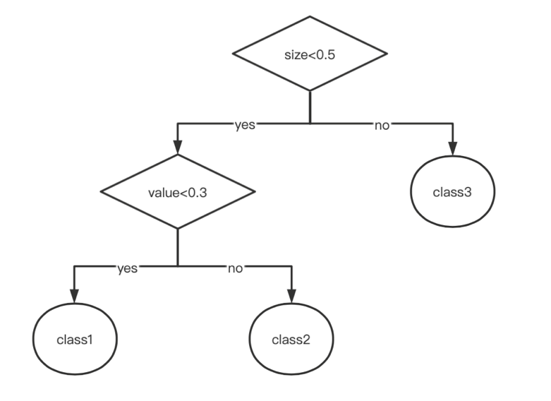
Figure 3: Regression tree example [1].

Selecting the optimal partition attribute is the critical point of tree model construction. Determining the optimal partition point can obtain the best branch effect while controlling the quality and quantity of features used can reduce the occurrence of over-fitting. We hope that the purer the information of the feature used to split the tree is, the better. For example, to judge whether to fly a kite, the weather attribute has a very high purity of information. In other words, the weather attribute is purer than the gender attribute for flying a kite. Because the sub features under the weather attribute can largely determine whether to fly a kite, for example, you must not fly a kite on rainstorm days. In 1984, Shannon proposed 'information entropy' as the most commonly used indicator to measure the purity of sample sets. Entropy represents the measurement of the uncertainty of random variables in information theory. The formula is:

\( Ent(D)=−\sum p∗logp \) (4)

The smaller the Ent (D) value, the higher the purity of the information represented and the better the effect of classification and regression. However, the prediction result of a single tree model is inferior when facing big data. Hence, people use the ensemble learning method to obtain a large number of basic tree models through different training methods, and the final model output is the summary of all the base tree prediction results. Integrated learning is divided into Bagging and boosting. The bagging voting method is to train multiple models and finally vote or average the prediction results of each model so that the results can be more accurate. Random Forest (RF) is a typical Bagging class integration algorithm. RF is an algorithm that integrates multiple decision trees. Each decision tree is a classifier, and N trees will have N classification results. The random forest will combine all results and specify the category with the most votes as the final output. The random forest model can be trained quickly and has good performance. In addition, there is the boosting class integration algorithm. Different from the Bagging method, it learns a model many times for learning the wrong samples many times. As a typical boosting integration model, XGboost performs well in many tasks.

5.2. Neural Network

In recent years, neural networks, especially the deep learning model, have been widely used in various fields and have performed very well, thanks to the rapid development of computer equipment and algorithms [15]. The classic neural network is a backpropagation neural network model, generally including the input, hidden, and output layers [4]. Data transmission at each layer will generate the following layer's data through the specified activation function. BP neural network is a neural network based on error backpropagation. In brief, the main difference between the neural network model and the linear model is the activation function, which makes the neural network model belong to the nonlinear model. Common activation functions include ReLU, sigmoid, tanh, et al. The ReLU function is used to calculate whether a number less than 0 is classified as 0 or not, which is the meaning of activation, which means the number can only be activated to participate in subsequent calculations if it is greater than 0. The network shown in the figure is realized by calculating the activation result several times, the formula is:

\( {h_{t}}=g(W_{x}^{(c)}{x_{t}}+ω_{0}^{(c)}) \) (5)

The model trained with samples will produce errors with the actual result value, which measures the effect of the model [16]. Back-propagation neural network is to propagate the error back into the model and continues to generate new model parameters. Multiple training will make the error smaller and smaller, which is also the main reason the neural network has a good prediction effect.

5.3. Recurrent Neural Network (RNN)

However, because the data samples are sent into the neural network one by one (see Figure 4), there is no mutual calculation process between the samples, and the order in which the samples are sent into the network has no impact on the prediction results [17].

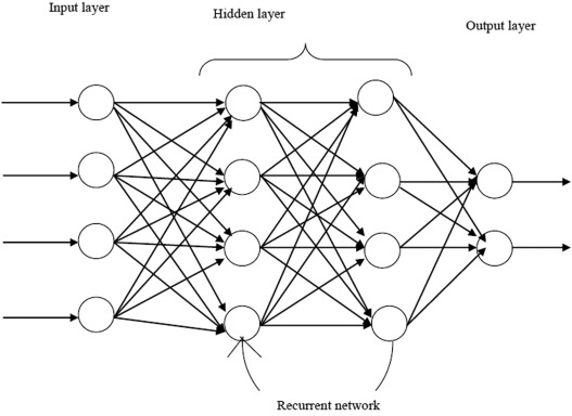
Figure 4: Recurrent neural networks [18].

While for financial data such as stocks, there is also time series information. The order of the samples contains information and cannot exchange positions. The sequence information has a prominent impact on the calculation results. Therefore, RNN, a deep learning model used in processing time series data, and the formula of objective function is:

\( {h_{t}}=g(W_{h}^{(c)}{h_{t−1}}+W_{x}^{(c)}{x_{t}}+ω_{0}^{(c)}) \) (6)

Compared with the ordinary neural network, there is one more item, , which is the accumulation of the calculation results of the last input sample [19]. RNN model performs very well in processing time series data. In addition, the combination of the recently emerging attention model and transformer model with financial topics is also worth trying [20].

6. Conclusion

This paper mainly introduces the feature processing-based machine learning asset pricing method and the end-to-end deep learning asset pricing method, reviews the existing methods and research progress of machine learning in the asset pricing field, and discusses the main problems encountered by the current machine learning asset pricing method. It could conclude that the integration of machine learning asset pricing method with modern information technology has great application potential.

However, data size is a limitation. With the increase of short samples and unstructured data, the time span of financial data is relatively short. For example, complete data on the U.S. stock market, even going back to 1970, is only about 600 monthly. These data are very limited to the large-scale training of machine learning and will affect the accuracy of the model. The role of non-traditional alternative data is more and more obvious, and migration algorithm is a possible solution. Many existing machine learning models do not consider the limiting factors of real transactions, such as asset liquidity, transaction costs, transaction friction and legal restrictions, etc. How to apply research results to specific business environments to supplement or replace human resources is an important research direction in the future.

References

[1]. Sharpe, W. F.: Capital asset prices: A theory of market equilibrium under conditions of risk. Journal of Finance 19(3), 425-442 (1964).
[2]. Ross, S. L.: The arbitrage theory of capital asset pricing. Journal of Economic Theory 13(3), 341–360 (1976).
[3]. Gu, S., Kelly, B. T., & Xiu, D.: Empirical Asset Pricing via Machine Learning. Review of Financial Studies 33(5), 2223–2273 (2020).
[4]. Gu, S., Kelly, B. T., & Xiu, D.: Autoencoder asset pricing models. Journal of Econometrics 222(1), 429–450 (2021).
[5]. Weigand, A.: Machine learning in empirical asset pricing. Financial Markets and Portfolio Management 33(1), 93–104 (2019).
[6]. Giglio, S., Kelly, B. T., & Xiu, D.: Factor Models, Machine Learning, and Asset Pricing. Annual Review of Financial Economics 14(1), 337–368 (2022).
[7]. Lettau, M., & Pelger, M.: Factors that fit the time series and cross-section of stock returns. The Review of Financial Studies 33(5), 2274-2325 (2020).
[8]. Jiang, J., Kelly, B. T., & Xiu, D.: (Re-)Imag(in)ing Price Trends. Social Science Research Network (2020).
[9]. Bagnara, M.: Asset Pricing and Machine Learning: A critical review. Journal of Economic Surveys (2022).
[10]. Jaggi, M.: An Equivalence between the Lasso and Support Vector Machines. In Chapman and Hall/CRC eBooks, pp. 19–44 (2013).
[11]. Support Vector Machine(SVM): A Complete guide for beginners. Analytics Vidhya. https://www.analyticsvidhya.com/blog/2021/10/support-vector-machinessvm-a-complete-guide-for-beginners/, last accessed 2023/4/20.
[12]. Bryzgalova, S., Pelger, M., & Zhu, J.: Forest through the trees: Building cross-sections of stock returns. SSRN (2020).
[13]. Coqueret, G., & Guida, T.: Machine Learning for Factor Investing : R version. In HAL (Le Centre pour la Communication Scientifique Directe). French National Centre for Scientific Research (2020).
[14]. Simonian, J., Wu, C., Itano, D., & Narayanam, V. R.: A Machine Learning Approach to Risk Factors: A Case Study Using the Fama–French–Carhart Model. The Journal of Financial Data Science 1(1), 32–44 (2019).
[15]. Yao, J., Li, Y., & Tan, C. L.: Option price forecasting using neural networks. Omega 28(4), 455-466 (2000).
[16]. Feng, G., He, J., & Polson, N. G.: Deep learning for predicting asset returns. arXiv preprint (2018).
[17]. Kumaraswamy, B.: Neural networks for data classification. In Elsevier eBooks pp. 109–131 (2021).
[18]. Chen, L., Pelger, M., & Zhu, J.: Deep Learning in Asset Pricing. Social Science Research Network (2019).
[19]. Drobetz, W., & Otto, T.: Empirical asset pricing via machine learning: evidence from the European stock market. Journal of Asset Management 22(7), 507–538 (2021).
[20]. Huang, J., Chai, J., & Cho, S.: Deep learning in finance and banking: A literature review and classification. Frontiers of Business Research in China 14(1), 1-24 (2020).
Cite this article
Zhao,F. (2023). A Literature Study of Asset Pricing Based on Machine Learning Method. Advances in Economics, Management and Political Sciences,34,27-36.
Data availability
The datasets used and/or analyzed during the current study will be available from the authors upon reasonable request.
Disclaimer/Publisher's Note
The statements, opinions and data contained in all publications are solely those of the individual author(s) and contributor(s) and not of EWA Publishing and/or the editor(s). EWA Publishing and/or the editor(s) disclaim responsibility for any injury to people or property resulting from any ideas, methods, instructions or products referred to in the content.
About volume
Volume title: Proceedings of the 7th International Conference on Economic Management and Green Development
© 2024 by the author(s). Licensee EWA Publishing, Oxford, UK. This article is an open access article distributed under the terms and
conditions of the Creative Commons Attribution (CC BY) license. Authors who
publish this series agree to the following terms:
1. Authors retain copyright and grant the series right of first publication with the work simultaneously licensed under a Creative Commons
Attribution License that allows others to share the work with an acknowledgment of the work's authorship and initial publication in this
series.
2. Authors are able to enter into separate, additional contractual arrangements for the non-exclusive distribution of the series's published
version of the work (e.g., post it to an institutional repository or publish it in a book), with an acknowledgment of its initial
publication in this series.
3. Authors are permitted and encouraged to post their work online (e.g., in institutional repositories or on their website) prior to and
during the submission process, as it can lead to productive exchanges, as well as earlier and greater citation of published work (See
Open access policy for details).