1. Introduction

The VIX is a widely used volatility index introduced by the Chicago Board Options Exchange, CBOE, in 1993. It is also known as the "Fear Index" or the "Fear Gauge [1]” since it reflects people’s anxiety over the market. The value of the VIX index tends to rise when there is increased uncertainty in the market. The VIX is calculated based on the prices of call and put option contracts of the SPX, which is the S&P 500 index, by aggregating the weighted average of those SPX option prices over a wide range of strike prices. It generates an expected volatility of the S&P 500 over the next 30 days.

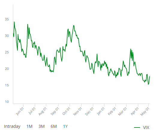
Figure 1: The Cboe volatility index®(VIX® index) from 2023 [2].

2. Methods

2.1. History of the VIX Index

The VIX has a history of almost 50 years. From its emergence to today, the VIX has become very common in the financial world. More and more people have become familiar with the VIX, which can be found everywhere in today's financial markets. Looking back at the history of the VIX, the Sigma index was first introduced in 1987 in an academic paper published by Brenner and Galai in the Financial Analysts Journal in July and August 1989. This is where the VIX was first noticed. Among others, Brenner and Galai wrote that "Our volatility index, to be named Sigma Index, would be updated frequently and used as the underlying asset for futures and options ... A volatility index would play the same role as the market index plays for options and futures on the index [3]". In 1992 after continuous research by Brenner and Galai, the American Stock Exchange announced a feasibility study of a volatility index and proposed the index as the "Sigma Index"[4]. Since then, research on the VIX has been on track. On March 19, 1993, the Chicago Board Options Exchange held a press conference to announce the launch of a real-time report on the CBOE Market Volatility Index, or VIX. The formula for determining the VIX is tailored to the CBOE S&P 100 Index (OEX) option price and was developed by Professor Robert E. Whaley [5]. The index measures implied volatility using a 30-day S&P 100 at-the-money [6]. 2003 - The CBOE introduces a new methodology for the VIX. Working with Goldman Sachs, the CBOE further develops the calculation and changes the underlying index for the CBOE S&P 100 Index (OEX) to the CBOE S&P 500 Index (SPX). This is now the algorithm for the VIX, a commonplace indicator of volatility expectations based on S&P 500 Index options. At this point, the algorithm update of the VIX index is complete. People began to trade a series of investments based on the VIX index. On March 26, 2004, VIX Index futures began selling for the first time on the Chicago Board Options Exchange (CFE) [7].

2.2. Key Moments of the VIX Index

The VIX index has also been used to assess the risk profile of financial markets after the final algorithm has been completed. Since it is an index, it is calculated based on the S&P 500 index. Since many social factors influence the S&P 500, the VIX will change whenever a turbulent event in history, especially a financial possibility.

Since 1993 the Chicago Board Options Exchange (CBOE) has introduced the VIX index as a measure of the expected volatility of the S&P 100 index. The VIX has been used to analyze financial markets. The following examples are good examples of how the VIX index changes after significant events. 27 October 1997: The VIX rose to its highest level in three years (above 35) due to the Asian financial crisis [8]. In 2002, a series of financial scandals, starting with Enron [9], pushed the VIX to 58 between July and November. 2008, when the subprime mortgage crisis erupted [10], the VIX reached 79 in October. 24 August 2015: The VIX rose sharply on the unexpected devaluation of the Chinese yuan [11]. 2018 Amid the financial meltdown [12], the VIX reached 50.30 points on February 6. 2020 February-March: the VIX spiked to a record high of 82.69 in response to the COVID-19 pandemic and its impact on global markets.

It is easy to see from these historical events that the VIX is subject to a variety of events, especially when there are financial events with global repercussions, and the VIX can change dramatically. At the same time, when the global economy is growing steadily, the VIX will remain at a relatively stable and small value. For example, the VIX index in May 2023 is around 18. On the other hand, if some global events occur, the VIX index will rise sharply, which means that the financial markets are unstable at that time, which is not conducive to the smooth development of the economy and investment.

3. Results and Discussion

3.1. Interpreting VIX Value

When VIX is high, it indicates that the market is expected to have greater volatility. When VIX is low, investors expect a more stable call. Hence, the VIX index and the SPX go in opposite directions. When the SPX value is high, the value of VIX is low, resulting in a stable market. Vice versa, when the SPX is low, the VIX tends to be increased due to high market turmoil [13]. The way of reading the VIX index depends on personal preference. However, the values of the VIX index can generally be divided into three categories. The First category is from 0 to 20, which indicates that the recent market is relatively stress-free and with little uncertainty. Under this range of values, investors do not need to worry about the risks that might be brought by market fluctuations when making decisions. The second category is from 20 to 30, which is a state where investors start to analyze the increasing uncertainty of the market. Making investment decisions becomes harder since many things need to be considered, such as whether this change in the value of VIX will be a short-term increase or a long-term effect or how much impact it will have if it keeps rising. When the value of the VIX index is above 30, the risks have increased to a certain level, and the market is experiencing a significant hit during this period. In total, the rise of the VIX value may be caused by various factors, such as changes in monetary policy, economic uncertainty, or political tensions.

3.2. Use of VIX

Therefore, The VIX index is often used for trading and hedging volatility [1]. For example, a trader might buy options to reduce losses when there is an expected increase in volatility, which means a high VIX value. Conversely, a trader might sell opportunities to gain income when the market is stable, shown by a low VIX value. The VIX index can also be viewed as an inverse indicator for some investors. When the VIX is high, some investors see it as a sign demonstrating an oversold market situation, so it may be an excellent time to buy.

Conversely, when the VIX is low, some investors see it as a sign of an overbought market, so it may be an excellent time to sell. The ways of interpreting the VIX index and reacting may vary depending on personal preference and experience, but overall, it is a frequently used indicator when making decisions. Moreover, the VIX index can also be used by economists and financial analysts to predict the market's future performance. Since it implies the level of stableness of the market, a bearish market is more likely to appear when there is a high VIX, while a low VIX value indicates a bullish market.

3.3. Trade and Products

The VIX index allows investors to gain advantages from the market changes expected by trading relative products. Since the VIX index is not tradable, it is sold through futures and options contracts or exchange-traded funds (ETFs) and exchange-traded notes (ETNs). Many of these products are highly liquid but also risky [13]. Examples of the products for trading relative to VIX are the iPath Series B S&P 500 VIX Short-Term Futures ETN (VXX), The iPath Series B S&P 500 VIX Mid-Term Futures ETN (VXZ), The ProShares Short VIX Short-Term Futures ETF (SVXY), and The ProShares VIX Mid-Term Futures ETF (VIXM) [14]. The VXX and the VXZ are ETNs issued by Barclays Capital. VXX has the characteristic of holding a long position in the first two months of daily rolling VIX futures contracts. VXZ is very similarly constructed to VXX but with longer-dated VIX future contracts. However, Contango, a common potential problem for future contracts where the future price is higher than the current price, also may occur here. Since there is an insurance premium for more extended warranties, VXX and VXZ commonly result in a lower return for long-term holders, making it more robust in the short term. The SVXY provides investors with daily inverse exposure to the VIX future contracts and benefits investors from the price difference resulting from the decline in prices within the day. The profits from SVXY usually occur in a stable or bullish market. Hence, there may be risks for long-term SVXY holders since they will see a significant loss when the market volatility increases suddenly. VIXM is provided for investors to hedge long-term market volatility rather than short-term volatility with which the VIX is primarily associated. This property of VIXM makes it valuable and effective for reducing the impact of Contango. Unlike the previous three examples suitable for short-term futures holders seeking profit from short-term market volatility, VIXM is ideal for investors with a low-risk tolerance or a long-term investment horizon [1].

4. Derivation of the VIX Index Formula

By using the Normal Standard deviation formula.

As we approach the VIX index by decomposition the general formula and then using the Normal Standard deviation formula to find the Standard deviation; as VIX is an index that shows the Volatility of the market thus, we suppose there is a relationship between the normal standard deviation and the VIX general formula. First, we get \( \frac{1}{T} \) from the general formula [15].

\( {σ^{2}}=\frac{2}{T}\sum _{i}^{n}\frac{∆{K_{i}}}{K_{i}^{2}}{e^{RT}}Q({K_{i}})-\frac{1}{T}{[\frac{F}{{K_{0}}}-1]^{2}}=\frac{1}{T}\lbrace 2 \sum _{i}^{n}\frac{∆{K_{i}}}{K_{i}^{2}}{e^{RT}}Q({K_{i}})-{[\frac{F}{{K_{0}}}-1]^{2}}\rbrace   \) (1)

\( (i=1,2,3…n) \)

Then we take the F (the forward index level derived from index option prices) to the function, which the F is calculated by: \( F=Strike price+{e^{RT}}×(Call price-Put price) \)

\( =\frac{1}{T}[2\sum _{i}^{n}\frac{∆{K_{i}}}{K_{i}^{2}}{e^{RT}}Q({K_{i}})-{(\frac{Strike price+{e^{RT}}×(Call price-Put price)}{{K_{0}}}-1)^{2}}]  \) (2)

\( (i=1,2,3…n) \)

Then we use the perfect square pattern to decompose the

\( {(\frac{Strike price+{e^{RT}}×(Call price-Put price)}{{K_{0}}}-1)^{2}}=\frac{1}{T}[2\sum _{i}^{n}\frac{∆{K_{i}}}{K_{i}^{2}}{e^{RT}}Q({K_{i}})]i=1,2,3…n -\frac{1}{T}{(\frac{Strike price+{e^{RT}}×(Call price-Put price)}{{K_{0}}})^{2}}-\frac{2}{T}(\frac{Strike price+{e^{RT}}×(Call price-Put price)}{{K_{0}}})+\frac{1}{T} \) (3)

we use the perfect square pattern again for

\( {(\frac{Strike price+{e^{RT}}×(Call price-Put price)}{{K_{0}}})^{2}} \) (4)

and split out the molecular of

\( 2(\frac{Strike price+{e^{RT}}×(Call price-Put price)}{{K_{0}}}) \)

\( =\frac{1}{T}[2\sum _{i}^{n}\frac{∆{K_{i}}}{K_{i}^{2}}{e^{RT}}Q({K_{i}})-\frac{Strike pric{e^{2}}}{K_{0}^{2}}-\frac{2 Strike price×{e^{RT}}×(Call price-Put price)}{{K_{0}}}] \)

\( -\frac{1}{T}[\frac{{e^{2RT}}{(Call price-Put price)^{2}}}{K_{0}^{2}}-\frac{2Strike price}{{K_{0}}}+\frac{2{e^{RT}}×(Call price-Put price)}{{K_{0}}}-1] \) (5)

Extract of common factorization of \( K_{0}^{2} \)

\( =\frac{1}{T}[2{e^{RT}}Q({K_{i}})\sum _{i}^{n}\frac{∆{K_{i}}}{K_{i}^{2}}-\frac{(Strike pric{e^{2}}-2Strike price×{K_{0}}+K_{0}^{2})}{K_{0}^{2}}]  \)

\( (i=1,2,3…n) \)

\( -\frac{1}{T}[\frac{2Strike price×{e^{RT}}×(Call price-Put price)×{K_{0}}+{e^{2RT}}{(Call price-Put price)^{2}}}{K_{0}^{2}}] \)

\( +\frac{1}{T}[\frac{2{e^{RT}}(Call price-Put price){K_{0}}}{K_{0}^{2}}] \) (6)

And use a perfectly square pattern for

\( (Strike pric{e^{2}}-2Strike price×{K_{0}}+K_{0}^{2}) \) (7)

\( =\frac{1}{T}[2{e^{RT}}Q({K_{i}})\sum _{i}^{n}\frac{∆{K_{i}}}{K_{i}^{2}}-{\frac{(Strike price-{K_{0}})}{K_{0}^{2}}^{2}}] \)

\( (i=1,2,3…n) \)

\( -\frac{1}{T}[\frac{{e^{RT}}(Call price-Put price)×(2Strike price×{K_{0}}-{e^{RT}}(Call price-Put price)+2{K_{0}})}{K_{0}^{2}}] \) (8)

Finally, we get the following formula

\( =\frac{1}{T}[2{e^{RT}}Q({K_{i}})\sum _{i}^{n}{\frac{∆{K_{i}}}{K_{i}^{2}}^{2}}](i=1,2,3…n) -\frac{1}{T}[\frac{{(Strike price-{K_{0}})^{2}}}{K_{0}^{2}}] \)

\( +\frac{1}{T}[\frac{({e^{RT}}×(Call price-Put price)(2Strike price×{K_{0}}-{e^{RT}}(Call price-Put price)+2{K_{0}}))}{K_{0}^{2}}] \) (9)

As we know, the standard deviation which is used to find the standard deviation of the multiple linear regression model is:

\( σ^{2}=\frac{\sum _{i=1}^{N}e_{i}^{2}}{n} \) (10)

As the T is time to expiration and VIX is calculated by the different days, thus T is the number of days we used. And \( e_{i}^{2} \) is the difference between the real and expected values or estimated values. Thus, we can see above \( 2{e^{RT}}Q({K_{i}})\sum _{i}^{n}\frac{∆{K_{i}}}{K_{i}^{2}} (i=1,2,3…n) \) is the real value we can get from the website, and

\( \frac{{(Sterile price -{K_{0}})^{2}}}{K_{0}^{2}}-\frac{[{e^{RT}}(Call price-Put price)(2Strike price×{K_{0}}-{e^{RT}}(Call price-Put price)+2{K_{0}})]}{K_{0}^{2}} \) (11)

is the estimated value or expected value. thus, we use the standard deviation approach to find the generalized formula used in the VIX Index calculation

5. Example for VIX Index Calculation on April 4th

Stock indices, such as the S&P 500, are market value-weighted indices of 500 major publicly traded companies in the United States. It is calculated using the prices of its constituent stocks. To determine the weight of each constituent stock in the S&P 500, the market capitalization of each company in the index is first added up, thus adding up the index's total market capitalization. Each of these indices uses rules to govern the selection of constituent securities and the formula for calculating the index value [1].

The VIX index is a volatility index. It differs from a stock index in that it is composed of options. And the price of each option reflects the financial market's expectations of future volatility. It's like financial markets weighing together all types of uncertainties to determine a forecast of future trends ultimately. It is more like digitizing the future of the financial markets with visual data to reflect whether the market is stable and worth investing in the future economy. Like traditional indices, the VIX Index is calculated using the rules for selecting component options and the formula for calculating the index value. Below is an example of how the VIX index is calculated.

The formula for the VIX index [15] is

\(  {σ^{2}}=\frac{2}{T}\sum _{i}^{n}\frac{∆{K_{i}}}{K_{i}^{2}}{e^{RT}}Q({K_{i}})-\frac{1}{T}{[\frac{F}{{K_{0}}}-1]^{2}}   (i=1,2,3…n) \) (12)

Note:

σ: VIX index/100=σ (Near-Month Volatility)

T: Time to expiration

R: Risk-free interest rate

S: the strike price at which the call option price differs the least from the put option price

F: S (Strike Price) + e^(RT) x (Call Price - Put Price)

\( {K_{0}} \) : the strike price that is less than F and closest to F

\( {K_{i}} \) : all strike prices from out-of-the-money option; (i=1,2,3 ....n). Call for \( {K_{i}} \) > \( {K_{0}} \) and Put for \( {K_{i}} \) < \( {K_{0}} \) , Put, and Call for \( {K_{i}} \) = \( {K_{0}} \) .

\( ∆{K_{i}} \) : Interval between strike prices. Usually, use half of the difference between either side of \( {K_{i}} \) . \( ∆{K_{i}} \) = \( \frac{|{K_{(i+1)}}-{K_{(i-1)}}|}{2} \)

\( Q({K_{i}}) \) : The midpoint of the bid-ask spread for each option with strike \( {K_{i}} \) .

The VIX Index measures the 30-day expected volatility of the S&P 500 Index, and the components of the VIX Index are calls and puts with expiration dates more significant than 23 days and less than 37 days. We can refer to them as "next-term" and "next-term." The next term is smaller than the next term.

In the following example, we will calculate the VIX index for April 15. To do this, we need two sets of data, one for the S&P 500 trike of May 12 (near-term) and the other for May 19 (next term). Both sets of data are available on the yahoo finance website.

First, The VIX index is calculated by measuring the time to expiration, T, in full days and dividing each day into minutes, which allows for more precision in professional options and volatility, thus making the data obtained more accurate. The following expression gives the time to expiration:

\( T=\frac{\lbrace {M_{Current day}}+{M_{Settlement day}}+{M_{Other day}}\rbrace }{ minutes in a year} \) (13)

\( {M_{Current day}} \) : How many minutes are left until midnight that day

\( {M_{Settlement day}} \) : minutes from midnight until 9:30 a.m. ET for “standard” SPX expirations

\( {M_{other days}} \) : total minutes in the days between the current day and the expiration day

In the above example, we have two sets of data, one is the near-term, and the other is the next-term. So, we need to compute two T-values.

T1= (846+510+40320)/525600=0.07929223744

T2= (846+900+48960)/525600=0.09647260273

Next, we need to calculate F. We will follow the formula of F to calculate the F value for both terms. Procedure F is shown below.

\( F=Strike price+{e^{RT}}×(Cell price-Put price) \) (14)

To find the strike price, we first need to compare the midpoint of the bid and ask which is smaller in the case of the same strike price of call and put. We have chosen 4135 as our strike price. This is for the near-term strike price and the same as the following-term price.

Near-term

Table 1: Prices of the near-term call options and mid-points of their bid and ask prices.

Table 2: Prices of the near-term put options and mid-points of their bid and ask prices.

Next-term

Table 3: Prices of the next-term call options and mid-points of their bid and ask prices.

Table 4: Prices of the next-term put options and mid-points of their bid and ask prices.

Then, we need to find the (call price - put price), the equal difference between the call midpoint and the put midpoint. The methods are the same for both the near and following terms.

Table 5: Difference between call and put mid-points for near-term and next-term.

After we find the strike price and (call price-put price), put all data in the F formula to get the F value for the near and next term. We take R to be 4%.

F1=4135+[e^(0.04*0.07929)]*19.425=4155.217749

F2=4135+[e^(0.04*0.09647)]*25=4160.096656

Third, Applying the VIX formula from the very beginning of this paper to the near-term and next-term options with expiration times T1 and T2, respectively, yields:

\( σ_{1}^{2}=\frac{2}{{T_{1}}}\sum _{i}^{n}\frac{∆{K_{i}}}{K_{i}^{2}}{e^{{R_{1}}{T_{1}}}}Q({K_{i}})-\frac{1}{{T_{1}}}[\frac{{F_{1}}}{{K_{0}}}-1]  i=1,2,3…n \) (15)

\( σ_{2}^{2}=\frac{2}{{T_{2}}}\sum _{i}^{n}\frac{∆{K_{i}}}{K_{i}^{2}}{e^{{R_{2}}{T_{2}}}}Q({K_{i}})-\frac{1}{{T_{2}}}[\frac{{F_{2}}}{{K_{0}}}-1]  i=1,2,3…n \) (16)

This formula looks complicated, so we will divide it into two parts, focusing first on the first half. It is

\( \frac{2}{{T_{1}}}\sum _{i}^{n}\frac{∆{K_{i}}}{K_{i}^{2}}{e^{{R_{1}}{T_{1}}}}Q({K_{i}})   (i=1,2,3…n \) )(17)

Table 6: The differences between call and put mid-points for near-term and next-term.

ΔKi is generally half the difference between the execution prices on either side of Ki. For the case of i=1, we choose the (i+1)th term minus the i-th period. For example, the first Put strike price on May 12th is 4000; since there is no price of the previous item, we choose the following data, which is 4005 minus 4000. Q(K )i is the midpoint of the bid-ask spread for each option with strike Ki.

Table 7: The contribution-by-strike for near-term and next-term.

After we have obtained the i-term values of k, Δk, and Q(k), we can sum them according to the equation. And derive the value of the first half of the σ formula.

s1= (2/0.07929)*0.00139=0.0351

s2= (2/0.09647)*0.002=0.0414

For the second half of the σ formula, K0 is the strike price less than F and closest to F.

y1=(1/T1)[(F1/K0)-1]^2=1/0.07929*(4155.217749/4135-1)^2=0.00030150613

y1=(1/T2)[(F2/K0)-1]^2=1/0.096472*(4160.096656/4135-1)^2=0.00038183822

After we obtain the two parts, we only need to calculate their difference to get the result to formula σ.

σ 1^2=s1-y1=0.0351-0.00030150613=0.03479849387

σ 2^2=s2-y2=0.0414-0.00038183822=0.04101816178

Lastly, we assign all the above data according to the VIX index formula, and we can get the result of the VIX index on April 15.

\( VIX=100×\sqrt[]{\lbrace {T_{1}}σ_{1}^{2}[\frac{{N_{{T_{2}}}}-{N_{30}}}{{N_{{T_{2}}}}-{N_{{T_{1}}}}}]+{T_{2}}σ_{2}^{2}[\frac{{N_{30}}-{N_{{T_{1}}}}}{{N_{{T_{2}}}}-{N_{{T_{1}}}}}]\rbrace ×\frac{{N_{365}}}{{N_{30}}}} \) (18)

\( {N_{{T_{1}}}} \) = number of minutes to a settlement of the near-term options (36000)

\( {N_{{T_{2}}}} \) = number of minutes to a settlement of the next-term options (48960)

\( {N_{30}} \) = number of minutes in 30 days (30 x 1,440 = 43,200)

\( {N_{365}} \) = number of minutes in a 365-day year (365 x 1,440 = 525,600)

\( VIX=100×\sqrt[]{\lbrace 0.07929*{0.0348^{2}}[\frac{48960-43200}{48960-36000}]+0.09647×{0.04102^{2}}[\frac{43200-36000}{48960-36000}]\rbrace ×\frac{525600}{43200}} \)

VIX = 16.72524782

This is the VIX index for April 15, calculated in the example above. After searching, we found that the actual VIX index of April 15 is 17, and it is easy to see that 16.725 is very close to 17. Some errors may be caused by the insufficient number of data sets selected; for example, we chose 60 data sets each for May 12 and May 19 and 30 sets each for call and put. This is more than enough, but perhaps more data would make the resulting VIX index more accurate.

After this example, two suggestions might be helpful in the subsequent VIX value calculation. The first is to choose as much data as possible when selecting data. This will result in a more accurate VIX calculation. As in the example above, only 60 sets of strike prices were chosen for each of the following and following terms. If more strike prices are selected, the results may be more accurate.

Secondly, one may wonder why not add more strike prices to make the VIX index in the above example more accurate. This is the second suggestion: never delete any data you have collected. In the example above, after finding two days of strike price data, we manually filtered 30 sets of calls and put data in each. And the data on the Yahoo finance site is updated in real-time every day, which makes it impossible for us to go back to April 15; once we delete any data, we can't get it back. So that's the second recommendation, it's best not to delete any of the strike price data you find, even if it's useless.

6. Conclusion

The VIX is a widely used volatility index that has become familiar since its introduction by the Chicago Board Options Exchange (CBOE) in 1993. To this day, the VIX index is an integral part of the financial markets. Systematically speaking, the VIX index can help us understand the future of financial markets and effectively assess the risk of investments. For calculating the VIX index in the example, there is a certain amount of error in the results. More data can be selected in the choice of the strike price to avoid such mistakes in the following calculation, thus further reducing the error. In the future, the application of the VIX index will be broader, and the research about the VIX index and derivative indexes needs to be further explored.

Acknowledgment

Muhao Hu, Gexuan Zhu, and Xinyu Wen contributed equally to this work and should be considered co-first authors.

References

[1]. Kenton, W. (2023, April 30). S&P 500 index: What it's for and why it's important in investing. Investopedia. Retrieved May 4, 2023, from https://www.investopedia.com/terms/s/sp500.asp
[2]. Cboe Global Markets. About Us. (n.d.). Retrieved May 4, 2023, from https://www.cboe.com/about/#our-story
[3]. Brenner, M., & Galai, D. (1989). New Financial Instruments for Hedging Changes in Volatility. Financial Analysts Journal, 45(4), 61–65. http://www.jstor.org/stable/4479241 doi:10.2469/faj.v45.n4.61
[4]. "IFR report" (PDF). people.stern.nyu.edu. 1992. Retrieved 2020-02-26 .https://pages.stern.nyu.edu/~mbrenner/research/IFR_report_on_Brenner-Galai_Sigma_Index.pdf
[5]. Mehta, Salil (July 2015). "Volatility in motion" (blog). Statistical Ideas. Retrieved 26 February 2020 – via Statisticalideas.blogspot.com
[6]. Volatility in motion. Statistical Ideas. (n.d.). Retrieved May 4, 2023, from http://statisticalideas.blogspot.com/2015/07/volatility-in-motion.html
[7]. Team, T. I. (2022, November 10). The impact of China devaluing the yuan in 2015. Investopedia. Retrieved May 4, 2023, from https://www.investopedia.com/trading/chinese-devaluation-yuan/
[8]. Michael Carson and John Clark. (n.d.). Asian financial crisis. Federal Reserve History. Retrieved May 4, 2023, from https://www.federalreservehistory.org/essays/asian-financial-crisis
[9]. Hayes, A. (2023, March 28). What was Enron? what happened and who was responsible. Investopedia. Retrieved May 4, 2023, from https://www.investopedia.com/terms/e/enron.asp
[10]. Duca, J. V. (n.d.). Subprime mortgage crisis. Federal Reserve History. Retrieved May 4, 2023, from https://www.federalreservehistory.org/essays/subprime-mortgage-crisis
[11]. Kuepper, J. (2023, March 20). Cboe volatility index (VIX): What does it measure in investing? Investopedia. Retrieved April 14, 2023, from https://www.investopedia.com/terms/v/vix.asp
[12]. staff, S. T. (2008, March 10). In the midst of a financial meltdown. The Seattle Times. Retrieved May 4, 2023, from https://www.seattletimes.com/opinion/in-the-midst-of-a-financial-meltdown/
[13]. Reiff, N. (2022, October 30). How to use a VIX ETF in your portfolio. Investopedia. Retrieved April 14, 2023, from https://www.investopedia.com/investing/use-vix-etf-in-your-portfolio/
[14]. Schwab.com. (n.d.). Vix etfs: The Facts and Risks. Schwab Brokerage. Retrieved April 14, 2023, from https://www.schwab.com/learn/story/vix-etfs-facts-and-risks
[15]. Volatility index®methodology: Selected broad-based index, equity and ... (n.d.-b). https://cdn.cboe.com/api/global/us_indices/governance/Volatility_Index_Methodology_Selected_Broad_Based_Index_Equity_and_ETF_Volatility_Indices.pdf.
Cite this article
Hu,M.;Zhu,G.;Wen,X. (2023). Research on the Development Trend and Application of VIX Index. Advances in Economics, Management and Political Sciences,37,42-54.
Data availability
The datasets used and/or analyzed during the current study will be available from the authors upon reasonable request.
Disclaimer/Publisher's Note
The statements, opinions and data contained in all publications are solely those of the individual author(s) and contributor(s) and not of EWA Publishing and/or the editor(s). EWA Publishing and/or the editor(s) disclaim responsibility for any injury to people or property resulting from any ideas, methods, instructions or products referred to in the content.
About volume
Volume title: Proceedings of the 7th International Conference on Economic Management and Green Development
© 2024 by the author(s). Licensee EWA Publishing, Oxford, UK. This article is an open access article distributed under the terms and
conditions of the Creative Commons Attribution (CC BY) license. Authors who
publish this series agree to the following terms:
1. Authors retain copyright and grant the series right of first publication with the work simultaneously licensed under a Creative Commons
Attribution License that allows others to share the work with an acknowledgment of the work's authorship and initial publication in this
series.
2. Authors are able to enter into separate, additional contractual arrangements for the non-exclusive distribution of the series's published
version of the work (e.g., post it to an institutional repository or publish it in a book), with an acknowledgment of its initial
publication in this series.
3. Authors are permitted and encouraged to post their work online (e.g., in institutional repositories or on their website) prior to and
during the submission process, as it can lead to productive exchanges, as well as earlier and greater citation of published work (See
Open access policy for details).