1. Introduction

With the development of technology, the combination of finance and computer science is becoming more and more important, and the application of big data technology in the financial field is becoming more and more extensive. In recent years, stock price forecasting research has become more demanding, and the development of stock price forecasting strategy with both high recognition accuracy and high efficiency has been an important task in the financial community. This paper discusses the implementation of LSTM-CNN-attention model. All the techniques are applied on the stock price dataset of French’s top smartphone corporation Alcatel Lucent. The main contribution of this research is to show that the attention mechanism increases the accuracy of the prediction.

This study manuscript will continue in the following structure. The second part provides a summary of related time series analysis literature. The procedures have been laid out in the third section. In the fourth section, experimental results have been shown and MSE has been computed. The effect on the attention Networks has also been discussed. Finally, the paper discusses the future work that can be done on stock price forecasting.

2. Related Works

2.1. Linear Method

Exponential smoothing is one of the early commonly used methods for time series data prediction, originated in the 1950s and 1960s [1]. It calculates the weight to show the relation between the real and forecast values and predicts with the weighted arithmetic average. This algorithm is simple to implement and requires little data information. It can predict the stock data at the next moment only by using the weighted sum of historical data. But limitations are following. First of all, it is sensitive to the smoothing coefficient. In addition, this method is only suitable for short-term forecasting, serious errors always appear for long-term and unstable stock data.

Slutsky, Walker, Yaglom, and Yule invented autoregressive (AR) and moving average (MA) models based on the premise that every time series is a stochastic process [1]. However, autoregressive integrated moving average model (ARIMA) with AR, MA is not appropriate for long-term prediction and is challenging to use for volatile market data [2]. Because the method is fundamentally to deal with stationary data, the performance can be effectively improved by combining nonlinear models.

2.2. Nonlinear Method

Financial time series exhibit volatility clustering, with high (low) absolute returns following each other. Engle devised autoregressive conditional heteroscedastic (ARCH) in 1982 to explain conditional variance changes as a quadratic function of historical returns. A more parsimonious model generalized ARCH (GARCH) was launched afterwards [1].

The rapid development of computer science and artificial intelligence has provided an opportunity to promote the progress in forecasting the stock price using machine learning algorithms. White [3] applied BP neural network to the stock forecast, but it is easy to fall into local minimum values. Lu et al. [4] used principal component analysis (PCA) to reduce data dimension, effectively simplify the input of network, so as to improve the speed of training. To avoid falling into local minimum value, Ji added momentum item into weight adjustment formula [1]. In addition, Li [5] and Guo et al. [6] introduced genetic algorithm to improve the method, which further alleviated the above problems.

RNN's temporal properties make it good for temporal data prediction. As an improvement, LSTM [7] overcomes gradient disappearance in RNN by skillfully combining short-term and long-term memory. Ning Xianbo et al. proposed LSTM-Adaboost. Kumar et al. used Adam optimizer to backpropagate LSTM recursive neural networks to predict NASDAQ stock prices.

3. Method

In this paper, the proposed LSTM-CNN-attention model is generated by adding a Squeeze-and-Excitation Network [11] to the CNN-LSTM construction. CNN-LSTM [8] which avoids the layback of LSTM and increases the robustness of CNN is built with pytorch, containing a Input layer, a Convolution layer, a Pooling layer, a Dropout function, a LSTM layer, and a Output layer as shown in Figure 1.

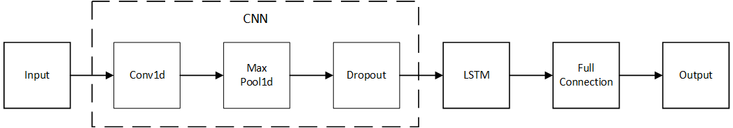
Figure 1: system construction.

Convolution layer: In this paper, Conv1d function is used to create a convolution layer, where stride is 1 without padding. Convolution kernel's size is 1*4.

Pooling layer: The pooling process always follows the convolution process to compress the feature map for higher calculation speed. The most commonly used pooling process is called Max pooling. In this paper, kernel size in MaxPool1d function is set as 5. If the input size is (n, C, Lin), the output (n, C, lout) is calculated as:

\( {L_{out }}=\frac{{L_{in}}+2× padding – dilation ×(kernel\_size-1)-1}{ stride }+1\ \ \ (1) \)

Dropout: Preventing feature detector dropout helps prevent overfitting and partially regularize. During forward propagation, dropout uses Bernoulli function to generate a vector of 0 or 1 for each neuron, 0 means that the neuron stops working. Here, the dropout ratio p is set to 0.01, which means 1% of hidden neurons are temporarily deleted during each iteration.

LSTM solves gradient vanishing. It learns long-term dependent knowledge easily. Figure 2 shows LSTM cells with three gates (forget gate, input gate, and output gate) and four activation functions (three sigmoid and one tanh). Unlike RNN, which use h_t to store short-term state, LSTM adds a parameter c to store long-term state, so that it makes up the defect in long-term forecasting.

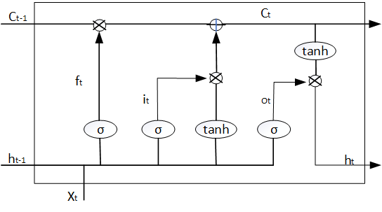
Figure 2: LSTM construction.

The Forget Gate is essentially a sigmoid layer, which looks at ht-1 and xt and outputs a number between 0 and 1:

\( {f_{t}}=σ({W_{f}}\cdot [{h_{t-1}},{x_{t}}]+{b_{f}}) \) (2)

Another sigmoid layer constitutes the Input Gate, transforming ht-1 and xt to it:

\( {i_{t}}=σ({W_{i}}\cdot [{h_{t-1}},{x_{t}}]+{b_{i}}) \) (3)

A tanh layer generates a vector \( {\widetilde{C}_{t}} \) :

\( {\widetilde{C}_{t}}=σ({W_{C}}\cdot [{h_{t-1}},{x_{t}}]+{b_{C}}) \) (4)

\( {\widetilde{C}_{t}} \) , it and ft take joint effort to get the state C at time t:

\( {C_{t}}={f_{t}}×{C_{t-1}}+{i_{t}}×{\widetilde{C}_{t}} \) (5)

Finally, the Output Gate runs a sigmoid function to decide ot:

\( {o_{t}}=σ({W_{o}}\cdot [{h_{t-1}},{x_{t}}]+{b_{o}}) \) (6)

Through a tanh layer, ot turns to a value between -1 and 1, which is multiplied to get state ht:

\( {h_{t}}={o_{t}}×tanh⁡({C_{t}}) \) (7)

Sigmoid mentioned above is a kind of activation function, which maps the sample value in the range of 0 to 1. The formula of sigmoid is as follows:

\( y=\frac{1}{1+{e^{-x}}} \) (8)

Hyperbolic tangent function (Tanh) mentioned above is another activation function:

\( tanh⁡(x)=\frac{sinh⁡(x)}{cosh⁡(x)}=\frac{{e^{x}}-{e^{-x}}}{{e^{x}}+{e^{-x}}} \) (9)

Squeeze-and-Excitation Networks [10] as shown in Figure 3 is added to the CNN-LSTM construction to form the LSTM-CNN-attention model. By learning the correlation between channels of the convoluted feature map, a one-dimensional vector is obtained as the evaluation score, each term in the vector corresponds each channel.

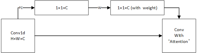
Figure 3: Squeeze-and-excitation networks.

4. Experiment

4.1. Data Exploration

The data set used in this paper is the stock price from 23 August 2016 to 23 August 2021 of Alcatel Lucent, a smartphone corporation from French. All 1280-row data is collected from Yahoo Finance. Data are ranked in time order, forming a time series.

There are serious variables: Date, Open, Low, High, Close, Adj Close, and Volume.

High, Low: the maximum and the minimum price on a particular trading day.

Open: the starting price on a particular trading day.

Close: the cash value of the last transacted price before the market closes.

After stock splits, dividends, and rights offers, the adjusted closing price shows a stock's value. Historical returns and performance analysis typically use it.

Volume: the number of shares traded.

Here is the head of the data set:

Table 1: The stock price of Alcatel Lucent from 23 August 2016 to 29 August 2016.

After importing the CSV file into spark, the count, mean, standard deviation, min, and max of the data set are shown in Figure 4:

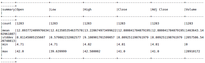
Figure 4: count, mean, standard deviation, min, and max of the data set.

The Pearson correlation is used to assess the correlation between the features [11], which ranges from 0 to 1. The closer the coefficient is to 1, the higher the correlation. As shown in Figure 5, Open, Low, High, Close, and Adj Close are highly positively correlated, so we only need to select one of them for analysis.

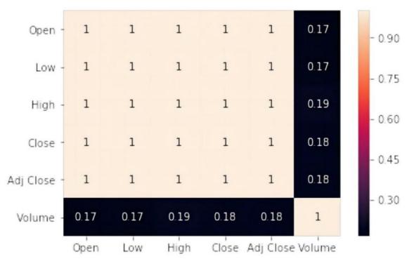
Figure 5: Correlation heat map.

In this paper, Adj Close is considered as the most important variable to experience, and the Matplotlib package is used to plot the graph of Adj Close over the entire timeline, as shown in Figure 6.

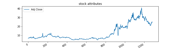
Figure 6: Visualization of Adj Close.

4.2. Time-Series Forecasting

4.2.1. Data Preprocessing

CSV files hold data. Normalization, filtering, and missing-value imputation must be done before data analysis. Normalization formula:

\( {X_{normal}}=\frac{X-{X_{min}}}{{X_{max}}-{X_{min}}}\ \ \ （10） \)

where \( {X_{normal}} \) is the normalized data, X is the original data, \( {X_{min}} \) and \( {X_{max}} \) are the minimum and maximum values among all data respectively.

To certify the accuracy of forecasting conveniently, the data set is split into two parts: the previous 90% is considered as training set, while the rest 10% is considered as test set to be predicted.

4.2.2. CNN-LSTM

Figure 7 illustrates the test set prediction result with the projected value in yellow and the true data in blue. It can be seen that the deviation is obvious.

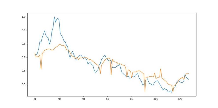
Figure 7: The predicted and real Adj Close price using CNN-LSTM [yellow:predict, blue:real].

4.2.3. CNN-LSTM-attention

In this part, the effect of attention is tested. By adding the Squeeze-and-Excitation Network in the model, a better result can be generated as Figure 8. It is easy to see that the predict line is closer to the true value.

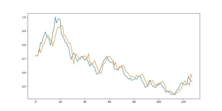
Figure 8: The predicted and real Adj Close price using CNN-LSTM-attention model.

4.3. Evaluation

The time-series data prediction task reduces the stock prediction data-historical data error. The model's training effect can be measured by mean square error (MSE):

\( MSE=\frac{\sum _{t=1}^{N}{(\hat{{x_{t}}}-{x_{t}})^{2}}}{N} \) (11)

where N represents the amount of time points, \( \hat{{x_{t}}} \) is the predicted value of stock data at time t, xt is the true value of stock data at time t.

In the experiment, the mean square error with the usage of CNN-LSTM model is 0.0048, adding attention mechanism declines the loss to 0.0016.

5. Conclusion

This paper compares the performance of time series forecasting models with and without attention on predicting the stock price. The conclusion is that the attention network can improve the accuracy of the prediction remarkably. Many factors can effect stock market prices, such as human manipulation and political involvement. The interaction between these components is also complicated. A more advanced approach is needed to anticipate the complex system with many affecting factors and uncertainty interactions.

References

[1]. Hyndman, R. J., & Ord, J. K. (2006). Twenty-five years of forecasting. International Journal of Forecasting, 22(3), 413 - 414.
[2]. Tingting, Z., H. Yajie, Y. Mengnan, R. Dehua, C. Yarui, W.Yuan, & L. Jianzheng (2021). Research review of time series data prediction method based on machine learning. Journal of Tianjin University of Science and Technology 36(5), page 9. 255
[3]. White (1988). Economic prediction using neural networks: the case of IBM daily stock returns. In: IEEE 1988 International Conference on Neural Networks, 451–458 vol.2.doi: 10.1109/ICNN.1988.23959.
[4]. Tianyu, L., D. Laina, W. Haiyuan, W. Yinqiu, T. Mingwan, & Z. Xuewu (2019). Prediction of stock price trend based on principal component analysis and neural network combination. Computer Knowledge and Technology: Academic Edition (2X), 4, 250.
[5]. Li, F. (2014). Research on Prediction Model of Stock Price 240 Based on LM-BP Neural Network. Proceedings of the International Conference on Logistics, Engineering, Management and Computer Science, Atlantis Press, pages 776–778.
[6]. Yiran, G. , & W. Xiuli (2019). Rotation prediction of stock 260 market size and cap style based on BP neural network. computer simulation, 36(3).
[7]. Sepp Hochreiter, & Jürgen Schmidhuber (1997). Long Short-Term Memory. Neural Comput, 9 (8), 1735–1780. doi: 10.1162/neco.1997.9.8.1735.
[8]. Taghavi Namin, S., Esmaeilzadeh, M., Najafi, M. et al. (2018). Deep phenotyping: deep learning for temporal phenotype/genotype classification. Plant Methods, 14, 66.
[9]. Bai, S., Kolter, J. Z., & Koltun, V. (2018). An empirical evaluation of generic convolutional and recurrent networks for sequence modeling. arXiv preprint arXiv:1803.01271.
[10]. Jie, Shen, Samuel, Albanie, Gang, Sun, and Enhua (2019). 235“Squeeze-and-Excitation Networks.” IEEE transactions on pattern analysis and machine intelligence.
[11]. Mohammed Ali Alshara (2022). Stock Forecasting Using Prophet vs. LSTM Model Applying Time-Series Prediction. IJCSNS, VOL.22 No.2.
Cite this article
Lyu,Z. (2023). Analysis and Time-series Forecasting of Corporate Stock Price. Advances in Economics, Management and Political Sciences,40,14-21.
Data availability
The datasets used and/or analyzed during the current study will be available from the authors upon reasonable request.
Disclaimer/Publisher's Note
The statements, opinions and data contained in all publications are solely those of the individual author(s) and contributor(s) and not of EWA Publishing and/or the editor(s). EWA Publishing and/or the editor(s) disclaim responsibility for any injury to people or property resulting from any ideas, methods, instructions or products referred to in the content.
About volume
Volume title: Proceedings of the 7th International Conference on Economic Management and Green Development
© 2024 by the author(s). Licensee EWA Publishing, Oxford, UK. This article is an open access article distributed under the terms and
conditions of the Creative Commons Attribution (CC BY) license. Authors who
publish this series agree to the following terms:
1. Authors retain copyright and grant the series right of first publication with the work simultaneously licensed under a Creative Commons
Attribution License that allows others to share the work with an acknowledgment of the work's authorship and initial publication in this
series.
2. Authors are able to enter into separate, additional contractual arrangements for the non-exclusive distribution of the series's published
version of the work (e.g., post it to an institutional repository or publish it in a book), with an acknowledgment of its initial
publication in this series.
3. Authors are permitted and encouraged to post their work online (e.g., in institutional repositories or on their website) prior to and
during the submission process, as it can lead to productive exchanges, as well as earlier and greater citation of published work (See
Open access policy for details).