1. Introduction

Since the 1980s, people have focused on stocks and securities in developed and emerging markets. In the last 30 years, there have been wider choices of assets and asset classes for asset allocation. However attractive the equity markets are from the standpoint of expected return, they also have considerable risks. From the Latin American debt crisis in the 1980s to the Technology bubble in 2000 and the Mortgage crisis of 2008, these examples illustrate how destructive the equity markets can be. To avoid repeating history repeatedly, we should learn historical lessons profoundly. This is why people are paying more and more attention to investment risk management and investment returns.

Portfolio theory is identified as the quantitative analysis of optimal risk management. As early as 1952, Markowitz [1] introduced the mean-variance theory, which pioneered using quantitative ideas to construct portfolios. Since then, there have been other scholars who have further investigated the Markowitz model. For example, Love et al. [2] attempted to develop a model based on the Markowitz model that would allow one to study the effect of diversification on export losses. Gollinger et al. [3] made the first attempt to calculate the efficient frontier of a commercial loan portfolio based on the structure of the Markowitz equity portfolio model. Shadabfar et al. [4] used a probabilistic approach to optimal portfolio selection using a mixture of Monte Carlo simulation and the Markowitz model.

To further refine the Markowitz model, William Shape [5] proposed the Single Index Model in 1963, which significantly promoted the practical application of portfolio theory. Other scholars have further investigated it since then. For example, Collins [6] used Single Index Model for risk analysis in farm planning applications. Galea et al. [7] studied structural Sharpe models under t-distribution. Mallikharjunarao et al. [8] constructed optimal portfolios in two sectors, sugar and metals, utilizing Sharpe index models.

On this basis, other scholars have compared these two models. For instance, Seler et al. [9] compared the Markowitz Mean-Variance Model and Sharpe Single Index Model to construct the Istanbul Stock Exchange portfolios for the period 1986-1987. Bekhet et al. [10] compared the Markowitz and single index models to construct portfolios of Amman Stock Exchange (ASE) companies. Finally, Susanti et al. [11] compare the best portfolio formation results of the Markowitz and single index models for LQ index 45 in the COVID-19 pandemic.

However, they do not sufficiently consider the practical use of the models. Therefore, we added a different constraint, i.e., whether to include the general index, to determine its effect on the two models. Furthermore, we tested the hypotheses of model normality and independence and compared the empirical results of the two models on this basis.

We select ten stocks from three industries over the past 20 years as samples. First, the Markowitz Model and the Index Model are used to construct portfolios with different constraints and test the assumptions of normality and independence of the models. After that, we compare the differences between the two models by calculating the corresponding feasible domains, i.e., the effective frontier, the ineffective frontier, and the minimum variance frontier, and two crucial points on the effective frontier, i.e., the minimum variance point and the maximum Sharpe point, and the Capital Allocation Line, and verify the reasonability of the results by combining Monte Carlo methods. Finally, we discuss the results of our models.

We organized the rest of the article as follows. An introduction to the theory of correlation models is provided in Section 2. Then, in Section 3, We preprocess the data and examine the normality of the actual data. In Section 4, we calculate and comparatively analyze the MM and IM model results. Finally, conclusions and future research directions are presented in Section 5.

2. Theory

2.1. The Full Markowitz Model (“MM”)

The Markowitz mean-variance model is based on the following assumptions.

(1) Investors consider each investment choice based on the probability distribution of security returns over the time of a given position.

(2) The investor estimates the risk of a portfolio based on the variance or standard deviation of the expected return of the security.

(3) The investor's decision is based solely on the risk and return of the security.

(4) At a certain level of risk, the investor maximizes the expected return; correspondingly, for a certain level of expected return, the investor minimizes the portfolio risk.

The expected return of the MM model portfolio \( p \) is:

\( {R_{p}}=\sum _{i=1}^{n}{w_{i}}{r_{i}} \) (1)

The standard deviation of the portfolio \( p \) is:

\( {σ_{p}}=\sqrt[]{\sum _{i=1}^{n}\sum _{j=1}^{n}{w_{i}}{w_{j}}cov({R_{i}},{R_{j}})} \) (2)

\( {r_{i}} \) : the expected return on asset \( i \)

\( {w_{i}} \) : represents the proportion of assets \( i \) in the portfolio

\( i \) : the number of total assets

\( cov({R_{i}},{R_{j}}) \) represents the covariance between the return on asset \( i \) and the return on asset \( j \)

2.2. Single Index Model (“IM”)

Two assumptions in William Sharpe’s single Index model.

(1) The securities risk is divided into systematic and idiosyncratic risk, and the factors (such as index) do not affect unsystematic risk.

(2) The idiosyncratic risk of one security does not affect the idiosyncratic risk of another, and the returns of the two securities are correlated only through the joint response of the factors.

The above two assumptions imply that \( cov{(}{R_{m}}{,}{ε_{i}})=0;cov{(}{ε_{i}},{ε_{j}})=0 \) , this simplifies the calculation to a large extent.

The expected return of the IM model portfolio \( p \) is

\( {R_{p}}=\sum _{i=1}^{n}{w_{i}}{r_{i}} \) (3)

The Standard deviation of Portfolio \( p \) is:

\( {σ_{p}}=\sqrt[]{(\sum _{i=1}^{n}{w_{i}}{β_{i}}{)^{2}}σ_{M}^{2}+\sum _{i=1}^{n}w_{i}^{2}{σ_{ε}^{2}}} \) (4)

\( {r_{i}} \) : the expected rate of return of asset \( i \)

\( {w_{i}} \) : denotes the proportion of asset \( i \) in the portfolio

\( n \) : the number of total assets

\( {β_{i}} \) : the risk factor of asset \( i \)

\( {σ_{M}} \) : systematic risk

\( {σ_{ε}} \) : unsystematic risk

2.3. Comparison Objects

• Minimum-Variance Frontier: this frontier is the curve traced by the portfolio point with the lowest variance at a given portfolio expected return. All individual assets are to the right of this boundary.

\( \begin{cases} \begin{array}{c} σ(\vec{w})→min{(}\vec{w}) \\ subject to:r(\vec{w})=const \end{array} \end{cases} \) (5)

• Minimal Return Frontier:

\( \begin{cases} \begin{array}{c} r(\vec{w})→min{(}\vec{w}) \\ subject to:σ(\vec{w})=const \end{array} \end{cases} \) (6)

• Efficient Frontier: all the points above the minimum variance portfolio on the minimum variance frontiers provide the optimal risk and return; therefore, they can be used as the optimal portfolio.

\( \begin{cases} \begin{array}{c} r(\vec{w})→max{(}\vec{w}) \\ subject to:σ(\vec{w})=const \end{array} \end{cases} \) (7)

• Global Minimal Risk Portfolio: the global Minimum-Variance frontier:

\( \begin{cases}σ(\vec{w})→\end{cases}min{(}\vec{w}) \) (8)

• Optimal Risky Portfolio: the tangential point of efficient frontier and CAL, it has Maximal Sharpe Ratio, which means maximal return, and lowest variance:

\( \begin{cases}\frac{r(\vec{w})}{σ(\vec{w})}→max{(}\vec{w})\end{cases} \) (9)

• Capital Allocation Line (CAL): a line is describing the relationship between expected return and risk for a portfolio of risky and risk-free investments. The slope of the CAL is called the Sharpe Ratio. This ratio measures the expected return in units of risk:

\( S=\frac{{E_{({R_{D}})}}-{r_{p }}}{{σ_{C}}} \) (10)

2.4. Normality Test

We select ten stocks from three different equity sectors (according to Yahoo Finance): technology, financial services, and industrials, to validate the model theory and use the S&P 500 as a market index (11 risky assets in total) and a proxy for a risk-free rate (1 month's federal fund's rate). We obtained the daily data of these stocks from May 11, 2001, to May 12, 2021, over the last 20 years using Bloomberg Professional. We further processed the data to include only five working days of daily data per week and produced the corresponding monthly data. First, we select ten stocks as a sample: ADBE, IBM, SAP, BAC, C, WFC, TRV, LUV, ALK, HA. Next, we use basic statistics, probability density functions, and Q-Q plots to compare the closeness of the daily and monthly data for ten stocks to a normal distribution to test the model's normality assumption. Next, we use basic statistics, probability density functions, and Q-Q plots to compare the closeness of the daily and monthly data for ten stocks to a normal distribution to test the model's normality assumption.

2.5. Statistical Comparison

We use Python to calculate the relevant statistical descriptions of each stock's daily and monthly data, and the results are shown in Table 1 and Table 2.

Table 1: Statistical information of daily stock data.

Table 2: Statistical information of monthly stock data.

Table 2: (continued).

Overall, the average monthly returns of individual stocks are larger and more volatile than the daily returns. Furthermore, the average skewness of the daily return of each stock is 0.43. On the other hand, the average kurtosis is 22.44, the average skewness of the monthly return is 0.11, and the average kurtosis is 4.40 (the skewness of the standard normal is 0, the kurtosis is 0). These indicate that the monthly data are closer to a standard normal distribution.

2.6. Comparison of All Stocks with Normal

Also, using Python, we plot histograms of daily and monthly returns for all 11 risky assets, along with their probability density curves and corresponding standard probability density curves, to compare the closeness of daily and monthly data to normality.

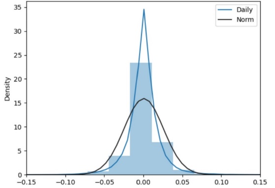
Figure 1: Comparison of daily data and normality.

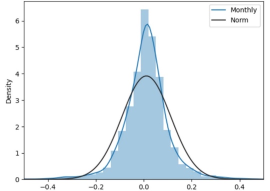
Figure 2: Comparison of monthly data and normality.

Comparing Figure 1 and Figure 2 shows that the monthly rate of returns data is closer to a normal distribution. The maximum probability density and the normal distribution are about 2, while the daily rate of return data differs by 20. Overall, the monthly data are closer to the average probability density.

2.7. Comparison of Each Stock with Normal

In order to further compare the closeness of each stock's daily and monthly returns to the normal distribution, we calculate the probability density value and the expected probability density function value of the corresponding point according to the histogram results and draw the corresponding curve for comparison.

The following is the formula for calculating the probability density values of the corresponding points based on the histogram results:

\( {P_{j}}=\frac{1}{Δr}\frac{{N_{j}}}{N} \) (11)

Where \( {P_{j}} \) is the probability density value corresponding to the \( j \) th interval, \( Δr \) is taken as 0.5%, \( {N_{j}} \) is the total number of returns for the \( j \) th interval, and \( N \) is the total number of returns.

For the daily data, our interval is chosen to cover three times the maximum standard deviation of each stock, which is about 12%. This means we can choose the following range of daily returns for the histogram.

\( r∈[-12\%,12\%] \) (12)

Using these formulas, the probability density of the daily rate of return, each stock's monthly rate, and its corresponding standard probability density value are calculated. Moreover, to better visualize the data and make the data more stable, we take the logarithm of the calculated probability density value. The comparison results of each stock with the normal distribution for daily data are shown in Figure 3.

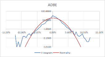
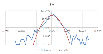
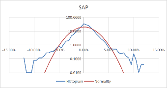
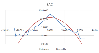
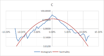
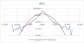
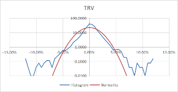
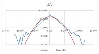
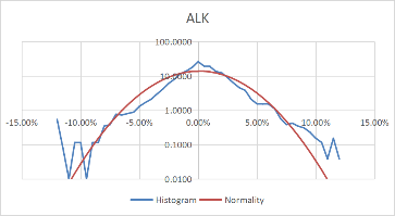
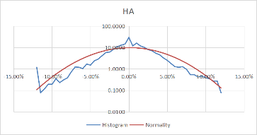
Figure 3: Comparison between stocks and normal for daily data.

For monthly data, because the standard deviation of each stock is more significant than the daily data, the interval selected at this time is to cover three times the average of the standard deviation of each stock, that is, a range for our histograms of monthly returns comes out to be approximately 29%. The comparison results of each stock with the normal distribution for monthly data are shown in Figure 4.

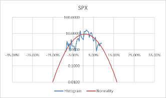
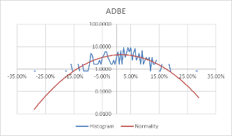
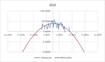
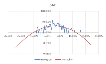
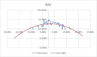
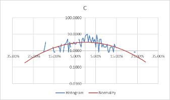
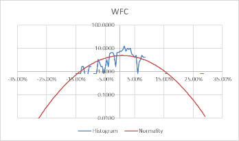
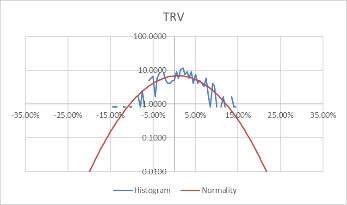
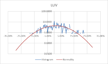
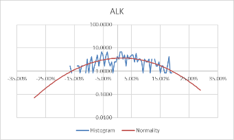
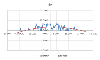
Figure 4: Comparison between stocks and normal for monthly data.

Comparing Figure 3 and Figure 4, it can be found that the monthly data is more concentrated in the middle than the daily data, and the fluctuation is relatively large. However, the overall distribution revolves around the standard probability density curve, and the difference from the normal is negligible. Moreover, the interval probability is smaller. We, therefore, conclude that the monthly data is more typical.

2.8. Comparison of the Q-Q Plots

After that, we used Python to draw Q-Q plots to analyze further the closeness of the daily and monthly return data to normality.

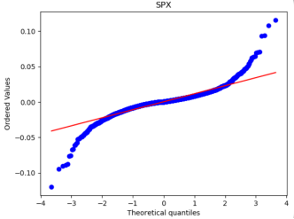
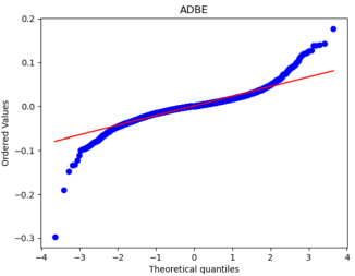
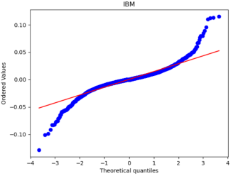
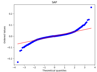
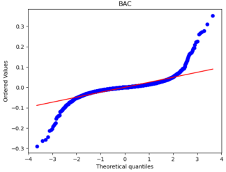
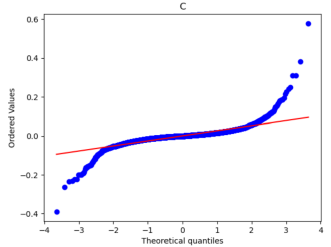
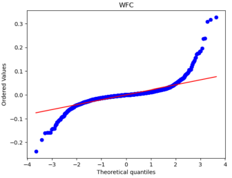
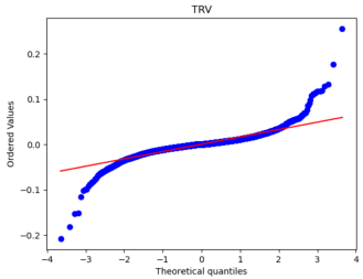
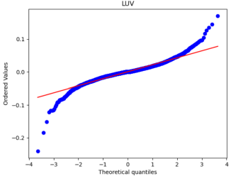
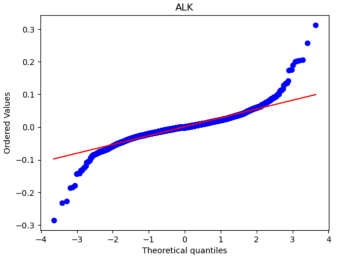
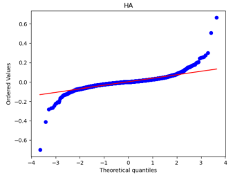
Figure 5: Q-Q plots of each stock’s monthly return.

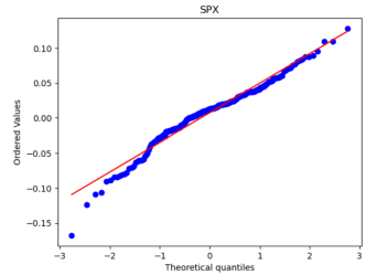
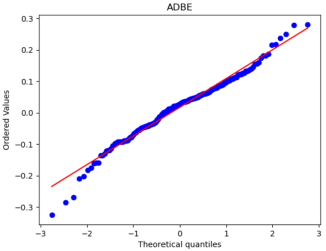
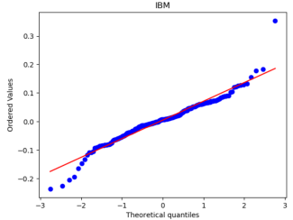
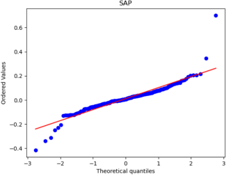
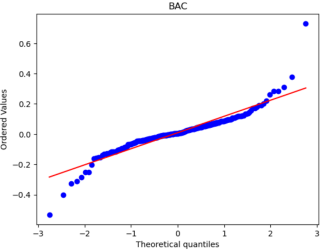
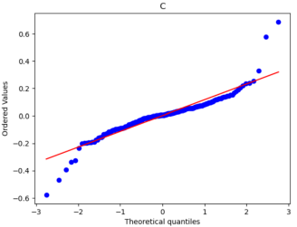
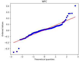
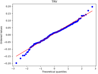
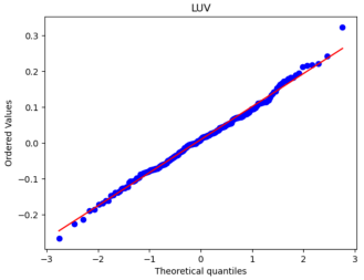
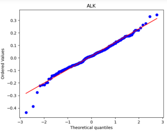
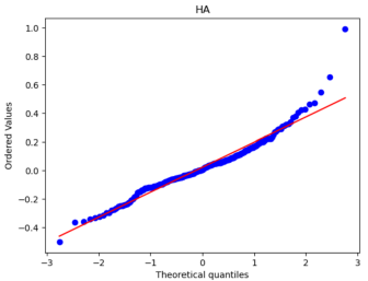
Figure 6: Q-Q plots of each stock’s daily return.

By comparing Figure 5 with Figure 6, it can be seen that the monthly data are distributed near a straight line. At the same time, the daily data, especially the two sections, are pretty different from the straight line, and the heavy-tailed distribution phenomenon is more pronounced. Therefore, it can be seen that the monthly returns of stocks are closer to a normal distribution.

Because one of the main assumptions of both the MM and IM models is that the securities returns obey the normal distribution to reduce the non-Gaussian effect and suppress the heavy-tailed distribution, our historical data is finally converted into monthly data closer to the normal distribution. However, it is different from a normal distribution.

2.9. Correlation Test

To test the independence assumption of the model, we plotted the heat map of correlation coefficients for each stock with the help of Python, as shown in Figure 7.

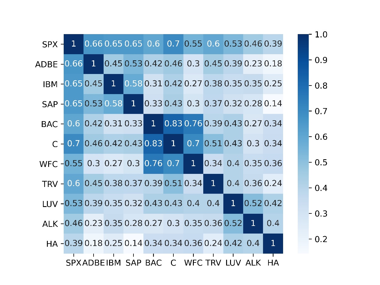
Figure 7: Correlation coefficients heat map.

It can be seen that stocks belonging to the same industry are highly correlated, especially stocks in the financial industry. BAC and C have the most significant correlation coefficient at 0.83, the strongest linear correlation, BAC and WFC are 0.76, and C and WFC stocks have a correlation coefficient of 0.7. At the same time, the SAP and HA correlation coefficients from different industries are at least 0.14. Most of the correlation coefficients are between 0.3-0.4, and the linear correlation is weak. As a whole, most stocks are relatively weakly correlated, except for a few pairs of stocks, but it can also be seen that the assumption of non-correlation is not always observed in practice.

3. Model Comparison

3.1. Calculation Inputs

We calculate all the required estimates for each of the optimization problems MM and IM based on monthly data by Solver. The result is shown in Table 3.

Table 3: Inputs results of the optimization problems.

After that, based on these model input values, we use SolverTable to calculate the permissible portfolio regions of the MM model and IM model composed of various portfolios under different constraints, namely the efficient frontier, the inefficient frontier, and the minimum variance frontier. Then we calculate two crucial points on the efficient frontier, namely the Global Minimal Variance points and Maximal Sharpe points (or Efficient Risky Portfolio), and the Capital Allocation Line to compare the differences between the two models.

3.2. Comparison of Two Portfolio

The results and weights of the portfolios constructed by the MM and IM models with minimum variance and maximum Sharpe ratio under two constraints are shown in Table 4 and Figure 8.

Table 4: Results of the portfolio with minimum variance and maximum Sharpe ratio.

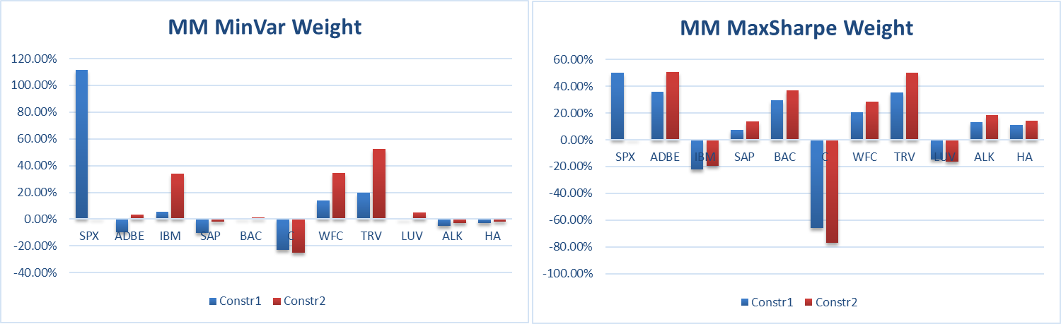
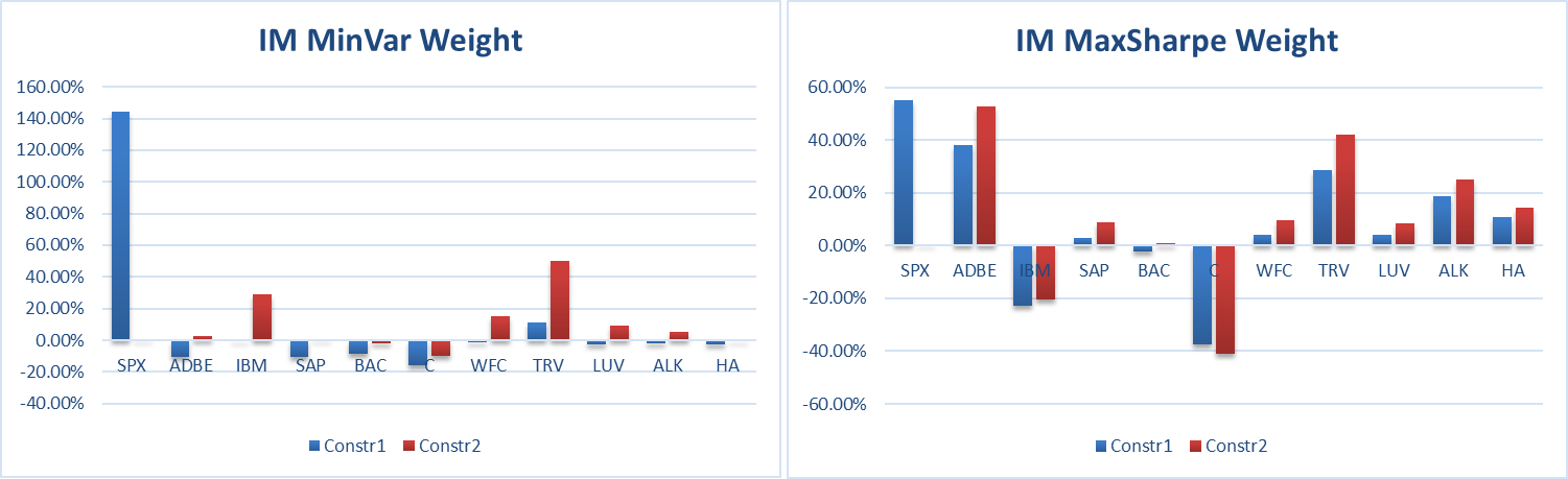
Figure 8: Weight Comparison.

Combining the results in Table 4 and Figure 8 shows that, when calculating the minimum variance portfolio, both models are more inclined to buy IBM, WFC, TRV stocks because of their smaller returns and standard deviations, short C, SAP stocks, and the IM model is in The SPX purchased under the condition of Constr1 will be about 30% more than that of the MM model. The proportion of other stocks will be reduced accordingly. However, the overall allocation ratio of each stock in the two models is similar, so the return of the minimum variance portfolio of IM will be less than the MM model. However, its standard deviation is slightly larger than the MM model, probably because the MM model as a whole allocates more funds to other stocks, which plays a role in diversifying risks.

When calculating the maximum Sharpe ratio portfolio, both models are more inclined to buy ADBE, SAP, WFC, TRV, ALK, and HA stocks and short IBM and C stocks because their returns and standard deviations are relatively small, and the overall can be seen that the asset allocation situation of the IM model is similar to that of the MM model. However, the SPX proportion purchased by the IM model under the condition of Constr1 is similar to that of the MM model, and the capital allocation of the remaining stocks is also similar to that of the MM model, except that the two stocks of BAC and LUV are long and short. Overall, the maximum Sharpe ratio portfolio of the IM model is closer to the MM model than the minimum variance portfolio.

To further quantify the differences between the two models at two points, we calculate the differences in portfolio returns, standard deviations, and Sharpe ratios for the minimum variance and maximum Sharpe ratios of the MM and IM models under different constraints. We calculated the differences between the corresponding values of the MM model and the IM model and then divided them by the values of the MM model and the results in Table 5 below.

Table 5: Point differences of MM and IM model.

Overall, IM is a better approximation of the MM model. the standard deviation of the IM model is closest to that of the MM model. At the same time, the Sharpe ratio differs the most from the MM model, and the returns also differ significantly. However, the returns for the two models with the slightest variance in the Constr2 condition are particularly close, and the Sharpe ratio difference is relatively small. In contrast, the standard deviation difference is considerable. Then, the differences in the bounds of the MM model and IM model under different constraints are calculated, and then the differences in the bounds of the two models are compared quantitatively. In this case, adding the general index, SPX, significantly impacts the portfolio. In this case, adding the general index, SPX, significantly impacts the portfolio.

Moreover, the minimum variance portfolio and the optimal portfolio constructed by Markowitz perform higher than the index model under the corresponding conditions, with higher returns, less risk, and a more excellent Sharpe ratio.

3.3. Comparison of the Two Optimization Problem Solutions under Different Constrain

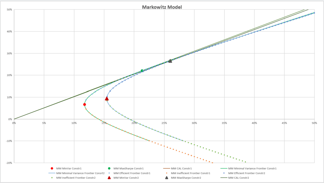
Figure 9: Comparison of different constraints of Markowitz Model.

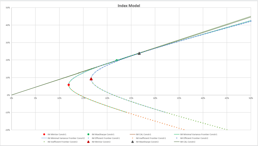
Figure 10: Comparison of different constraints of the Index Model.

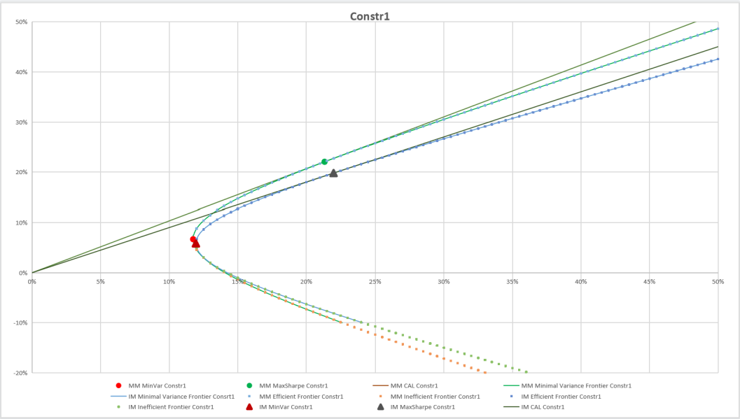
Figure 11: Comparison of different models under constr1.

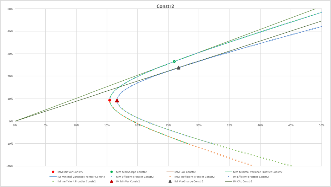
Figure 12: Comparison of different models under constr2.

Figure 9 and Figure 10 illustrate the comparison between the Markowitz and Index models with SPX (Constr1) and without SPX (Constr2) restrictions, respectively. Figure 11 and Figure 12 indicate the differences between Markowitz and IM models in the same constraint.

The four models have the following commonalities, the minimum variance portfolio and the maximum Sharpe ratio portfolio of Constr1 are both located on the upper right-hand side of Constr2. Compared to Constr1, Constr2 excludes SPX, which has a smaller average annual return and annual standard deviation than the ten stocks as a whole. Therefore, a portfolio with the minimum variance and maximum Sharpe ratio of the general index SPX removed will have greater relative returns and risk. The boundaries in the Constr1 condition, including the minimum variance, will enclose Constr2 and contain more area.

For the effective frontier, when the standard deviation is less than 25%, the return corresponding to the same standard deviation Constr1 will be more considerable. On the other hand, for the same return, the standard deviation corresponding to Constr1 will be smaller, indicating that the effective frontier constructed by introducing the general index SPX will be better. However, as the standard deviation increases, the practical boundaries under the two conditions become closer and closer, and the difference is not very obvious. Therefore, the effect of introducing the market index SPX on the effective frontier is not significant.

For the ineffective frontier, the return corresponding to Constr1 will be lower for the same standard deviation. In contrast, the standard deviation of Constr1 will be minor for the same return. The ineffective frontier under the two restrictions is parallel, indicating that the introduction of SPX has some influence on the ineffective frontier.

As for the CAL line, because the maximum Sharpe ratio in the Constr1 condition will be larger and the slope is more remarkable, its line will be above Constr2, and the maximum Sharpe ratio portfolio will more likely be in the upper right of Constr2. However, the overall difference between the two is insignificant, and the introduction of SPX does not significantly impact CAL.

3.4. Comparing the Quantitative Differences between the Two Models under Different Constraints

By calculating the difference between the frontiers of the MM model and the IM model under different constraints, the difference between the two models can then be compared quantitatively.

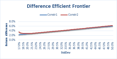
Figure 13: The efficient frontier difference between MM and IM model.

The difference between the efficient frontier of the two models under different constraints is compared by calculating the difference between the maximum returns of the two models with a given standard deviation. The results are shown in Figure 13. Overall, the difference between the practical boundaries of the two models is relatively similar under different constraints, and the two lines overlap. With the increase in standard deviation, the difference between the two models' returns under the two restriction conditions keeps increasing. When the standard deviation is less than 18.5%, the error of the effective frontier of the two models under the Constr2 condition increases. However, the overall error is small and stable within 2%-7%, indicating that IM is a better approximation of the MM model in terms of the effective frontier.

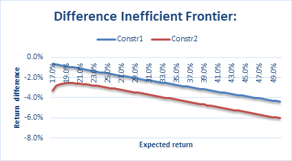
Figure 14: The inefficient frontier difference between MM and IM model.

By calculating the difference between the minimum returns of the two models under a given standard deviation, the difference between the ineffectiveness bounds under different constraints is compared, and the results are shown in Figure 14. Overall, the different curves of the two models' ineffective boundaries are parallel. The difference between the two models' returns under the two restriction conditions keeps increasing as the standard deviation increases. The difference between the ineffective boundaries of both models under the Constr2 condition is more significant than that under the Constr1 condition. For the ineffective frontier, the different curves of the two models in both conditions are less than 0, indicating that the minimum return corresponding to the ineffective frontier of both IM models will be greater than that of the MM model. However, the overall error is minor, basically stable at -6% to 0%, indicating that IM is a better approximation of the MM model under the ineffective frontier. Overall, the difference between the two models for the ineffective frontier will be smaller than the effective boundary.

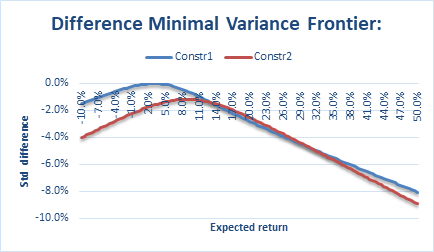
Figure 15: The minimal variance frontier difference between MM and IM model.

The difference between the minimum standard deviation of the two models for a given expected return is calculated to compare the difference in the minimum variance frontier between the two models under different constraints. The results are shown in Figure 15. Overall, as the expected return increases, the difference between the two models under both constraints decreases and increases, and both curves are less than 0. This indicates that the minimum variance bound of the MM model under both conditions corresponds to a smaller return value than the IM model. For example, for a given expected return of 12.5% to 32.5%, the difference between the minimum variance bounds of the two models under the Constr2 condition will be smaller than Constr1. At the same time, outside this interval, the difference between the minimum variance bounds of the two models under the Constr1 condition will be enormous. As the absolute value of the given expected return increases, the difference between the two models between the two constraints also increases (the two-curve distance expands). However, the overall difference in the minimum variance boundaries of the two models under the Constr2 condition will be more significant than that of Constr1. However, the error range of the two models under different conditions is between -10% and 0%, slightly larger than the error range of the practical and invalid boundaries. However, the overall error is minor, indicating that the IM model is a better approximation of the MM model at the minimum variance frontiers.

3.5. Monte-Carlo

Monte-Carlos a numerical simulation method that takes probability phenomena as the research object. It is a calculation method for estimating unknown characteristic quantities by obtaining statistical values according to the sampling survey method. The Monte Carlo method is used to simulate the possible portfolio points generated for the MM and IM models, and the results are shown in Figure 16 and Figure 17.

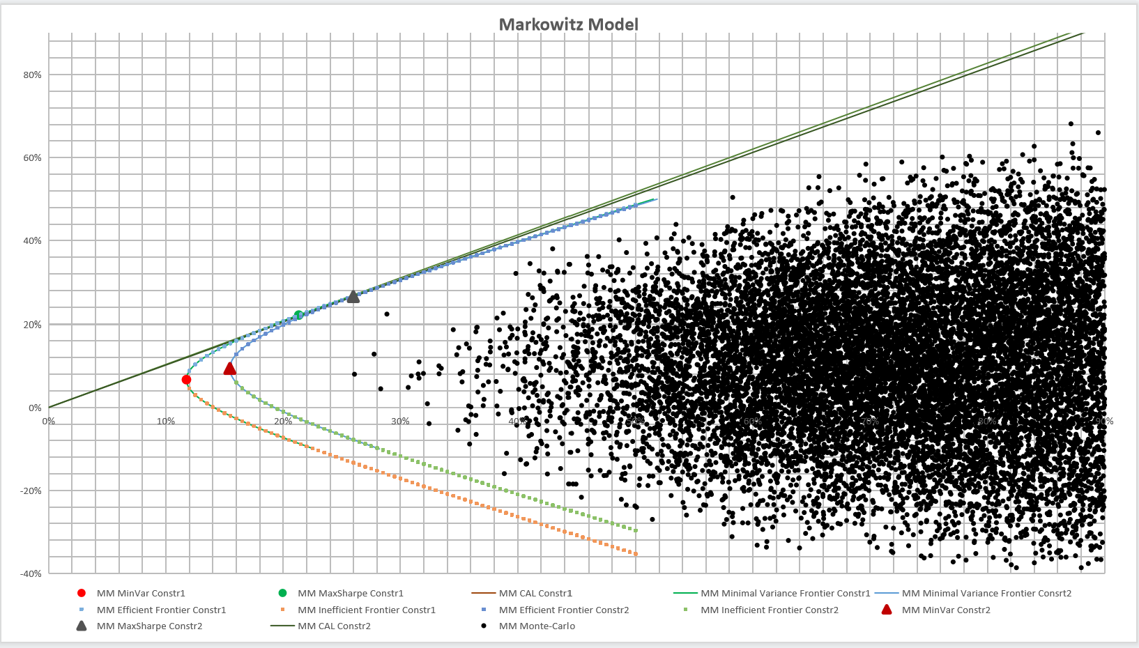
Figure 16: Monte Carlo of Markowitz model.

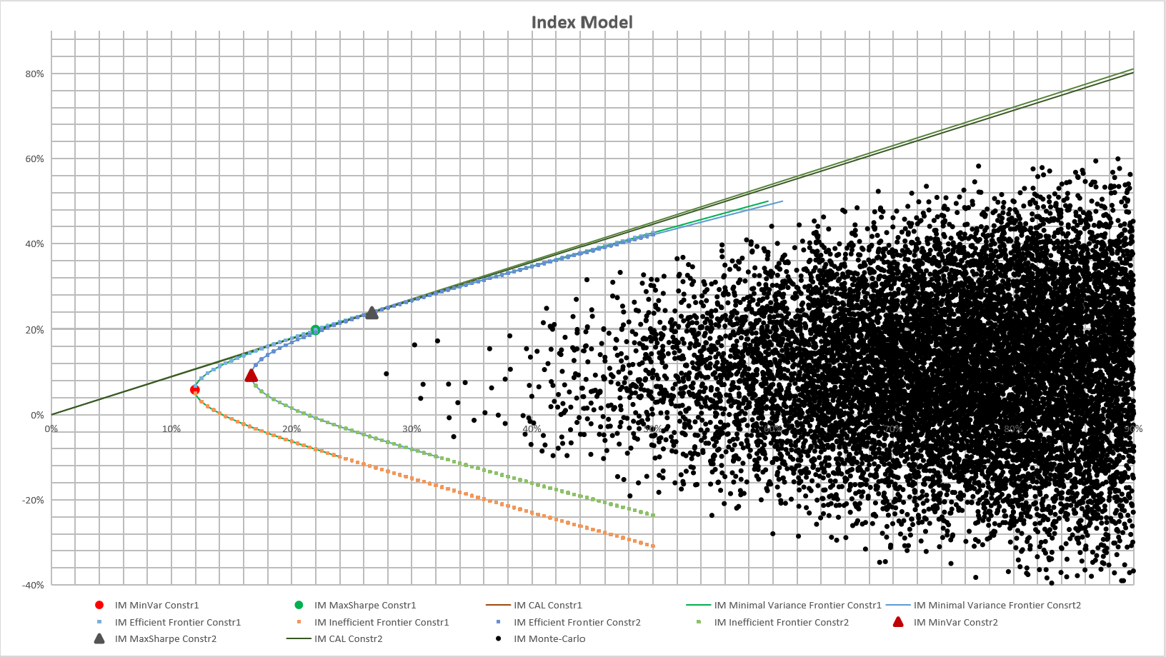
Figure 17: Monte Carlo for Index Model.

According to the Monte Carlo results in Figure 16 and Figure 17, it can be seen that the points simulated by Monte Carlo are within the feasible domain, indicating that the model data are reasonable.

4. Conclusion

4.1. Result and Analysis

Risk management is one of the essential parts of portfolio management. After identifying and assessing the risk, we need to analyze the portfolio's asset allocation further to minimize the risk with the same return. This article selected ten stocks from three sectors to compare the MM and IM models.

After that, we proceed to test the model hypotheses. First is the normality examination. We use the basic statistical information, probability density function, and Q-Q plot to compare the proximity of daily and monthly data of the ten stocks to the normal distribution and then choose to transform the data into monthly data, which is closer to the normal distribution, but it still differs from the normal distribution. Next is the correlation test. When calculating the correlation coefficients, we find that the correlation is more robust for stocks belonging to the unified industry, especially stocks in the financial sector. It shows that under realistic conditions, the assumptions of normality and correlation of the two models are not always satisfied.

Then, by contrasting the outcomes of the MM and IM models under different constraints, we find that although some models' assumptions are not met, the IM model is still a better approximation of the MM model. The MM model slightly outperforms the IM model, and the introduction of the general index SPX affects the results of both models to some extent. This is consistent with the results of some research scholars. For example, Bekhet et al. [10] found no significant difference between the tested models constructed with Markowitz and single index models for Amman Stock Exchange (ASE) companies. Yuwono et al. [12] found that the optimal portfolio return levels of listed stocks on the Jakarta Islamic Index of Indonesia Stock Exchange using Markowitz and single index models were insignificant. However, it is worth mentioning that different scholars have empirically tested the two models with different results. For example, Chasanah et al. [13] found that based on the M-V criterion, the optimal portfolio formed using the Markowitz model is superior to the single index model for the Jakarta Islamic Index (JII) stocks. Putra et al. [14] conducted an empirical test on the Indonesian stocks included in the LQ45 index of the stock exchange. They found that using a single index model performs better than the Markowitz model. Chen et al. [15] found that the Markowitz model performs better in high-risk portfolios and that using an index model would be a better choice for investors when faced with low-risk investment projects. It can be seen that based on different actual data, the portfolios constructed by the two models perform differently. Therefore, choosing the more appropriate model to construct the portfolio is ultimately essential based on the actual data.

To conclude, we conducted simulations using Monte Carlo methods and discovered that the generated points are within the feasible region, indicating that the sample results are reasonable.

Our study can further diversify the related research on Markowitz portfolios theoretically. However, at the same time, it can prevent investors from using historical data to estimate the future returns and risks of portfolios in practical investment activities, lower investors' investment risks, and provide some investment comments and suggestions for investors to construct and hold portfolios.

4.2. Limitations and Future Research

Our research only selected ten stocks in three less correlated sectors with a limited sample. It was found that neither the model's normality nor the uncorrelated assumptions were satisfied in the actual data, so the conclusions drawn can only be informative. For future research, we can try to combine multiple sectors and combine more other investment instruments, such as bonds, and funds, to obtain more reliable conclusions.

Second, in our study, we focus on comparing the MM model and the IM model. However, portfolio models need to include more, such as the mean-semivariance model, the mean-variance-skewness model, and the CAPM model for further comparative analysis.

Moreover, many risk indicators have certain limitations and conditions of use. For example, the Markowitz model can be used only with the expected return and the correlation of the securities, which requires many parameters and is difficult to obtain. The Sharpe index needs to be applied under the premise of a normal distribution, and as we can see from the graphs we have drawn, the returns of many stocks in real life are generally not distributed.

Even though there is a cost in risk control when investing for companies and individuals, the cost of not having reasonable risk avoidance will be higher.

Acknowledgment

Lin Cai, Yueying Jiang, and Yun Du contributed equally to this work and should be considered co-first authors.

References

[1]. Markowitz H. portfolio selection [J]. The journal of finance, 1952: 7 (1).
[2]. Love J. A model of trade diversification based on the Markowitz model of portfolio analysis[J]. The Journal of Development Studies, 1979, 15(2): 233-241.
[3]. Gollinger T L, Morgan J B. Calculation of an efficient frontier for a commercial loan portfolio[J]. Journal of Portfolio Management, 1993, 19(2): 39.
[4]. Shadabfar M, Cheng L. Probabilistic approach for optimal portfolio selection using a hybrid Monte Carlo simulation and Markowitz model[J]. Alexandria engineering journal, 2020, 59(5): 3381-3393.
[5]. Sharpe W F. A simplified model for portfolio analysis[J]. Management science, 1963, 9(2): 277-293.
[6]. Collins R A, Barry P J. Risk analysis with single‐index portfolio models: An application to farm planning[J]. American Journal of Agricultural Economics, 1986, 68(1): 152-161.
[7]. Galea M, Cademartori D, Vilca F. The structural Sharpe model under t-distributions[J]. Journal of Applied Statistics, 2010, 37(12): 1979-1990.
[8]. Mallikharjunarao T, Anithadevi S. CONSTRUCTION OF OPTIMAL EQUITY PORTFOLIO WITH APPLICATION OF SHARPE SINGLE INDEX MODEL: A COMPARATIVE STUDY ON FMCG AND AUTO SECTORS[J]. CLEAR International Journal of Research in Commerce & Management, 2017, 8(8).
[9]. Seler İ T. Portfolio Selection Methods: an Application to İstanbul Securities Exchange[D]. Bilkent Universitesi (Turkey), 1989.
[10]. Bekhet H A, Matar A. Analyzing risk-adjusted performance: Markwoitz and single index approaches in Amman Stock Exchange[C]//International Conference on Management (ICM) Proceeding. 2011: 305-321.
[11]. Susanti E, Ervina N, Grace E, et al. Comparison Analysis Of Optimal Portfolio Formation Results Using Single Index Model With Markowitz Model During The Covid 19 Pandemic In LQ 45 Index Company[J]. International Journal of Educational Research & Social Sciences, 2021, 2(5): 1146-1156.
[12]. Yuwono T, Ramdhani D. Comparison Analysis of Portfolio Using Markowitz Model and Single Index Model: Case in Jakarta Islamic Index[J]. Journal of Multidisciplinary Academic, 2017, 1(1): 25-31.
[13]. Chasanah S I U, Lesmana D C, Purnaba I G P. Comparison of The Markowitz and single index model based on MV criterion in optimal portfolio formation[J]. International Journal of Engineering and Management Research (IJEMR), 2017, 7(4): 323-328.
[14]. Putra I, Dana I M. Study of Optimal Portfolio Performance Comparison: Single Index Model and Markowitz Model on LQ45 Stocks in Indonesia Stock Exchange[J]. American Journal of Humanities and Social Sciences Research (AJHSSR), 2020, 3(12): 237-244.
[15]. Chen Z, Li H, Li Z, et al. Analysis of Ten Stock Portfolios Using Markowitz and Single Index Models[C]//2022 7th International Conference on Social Sciences and Economic Development (ICSSED 2022). Atlantis Press, 2022: 1219-1225.
Cite this article
Cai,L.;Jiang,Y.;Du,Y. (2023). Comparison of Markowitz Model and Index Model in Capital Markets. Advances in Economics, Management and Political Sciences,5,137-158.
Data availability
The datasets used and/or analyzed during the current study will be available from the authors upon reasonable request.
Disclaimer/Publisher's Note
The statements, opinions and data contained in all publications are solely those of the individual author(s) and contributor(s) and not of EWA Publishing and/or the editor(s). EWA Publishing and/or the editor(s) disclaim responsibility for any injury to people or property resulting from any ideas, methods, instructions or products referred to in the content.
About volume
Volume title: Proceedings of the 2022 International Conference on Financial Technology and Business Analysis (ICFTBA 2022), Part 1
© 2024 by the author(s). Licensee EWA Publishing, Oxford, UK. This article is an open access article distributed under the terms and
conditions of the Creative Commons Attribution (CC BY) license. Authors who
publish this series agree to the following terms:
1. Authors retain copyright and grant the series right of first publication with the work simultaneously licensed under a Creative Commons
Attribution License that allows others to share the work with an acknowledgment of the work's authorship and initial publication in this
series.
2. Authors are able to enter into separate, additional contractual arrangements for the non-exclusive distribution of the series's published
version of the work (e.g., post it to an institutional repository or publish it in a book), with an acknowledgment of its initial
publication in this series.
3. Authors are permitted and encouraged to post their work online (e.g., in institutional repositories or on their website) prior to and
during the submission process, as it can lead to productive exchanges, as well as earlier and greater citation of published work (See
Open access policy for details).