1. Introduction

With the rapid development of communication applications, communication technology is constantly experiencing revolutionary iterations. From the First Generation (1G) analog communication system to the Fifth Generation (5G) digital communication system, each upgrade is accompanied by an increase in frequency, an expansion of bandwidth, and a significant increase in data transmission rate [1]. In order to cope with the increasingly complex communication scenario requirements, signal modulation methods have become more and more complex and diverse, which undoubtedly brings unprecedented challenges to the research of signal modulation recognition technology [2]. Therefore, Automatic Modulation Recognition (AMR) plays a vital role in modern wireless communication systems and is mainly used to identify the modulation method of wireless signals.

Automatic modulation recognition has a wide range of uses in both military and civilian fields. AMR can identify and receive signals in non-cooperative communication without knowing the corresponding modulation method. This application provides conditions for information acquisition in certain situations. In the military field, it can be used to analyze and interfere with enemy signals, search and capture enemy targets, and evaluate and warn battlefield situations; in the civilian field, it can be used for adaptive coding, spectrum monitoring, spectrum management, etc. [3].

The implementation of AMR requires the processing of a large amount of data. In recent years, with the advancement of computer hardware, Graphics Processing Units (GPU) have provided extremely powerful floating-point computational efficiency, enabling the use of Deep Learning (DL) neural networks in AMR.

This paper primarily describes the recognition accuracy of AMR using a Convolutional Neural Network (CNN) with two convolutional layers under various channel conditions, followed by the introduction of Long Short-Term Memory (LSTM) networks. By combining the advantages of both LSTM and CNN, a hybrid neural network is developed to optimize AMR accuracy while simultaneously improving computational speed.

2. Principle overview

2.1. Basic principles of AMR

AMR is a technology that automatically determines the modulation mode of a received radio signal by analyzing it. Its core goal is to complete classification based only on signal waveform features without prior knowledge (such as modulation type, symbol rate, etc.). The AMR process works as follows: first, a data set is obtained, then data preprocessing is performed, and feature extraction and classification are performed on this basis, and finally, the corresponding modulation style is obtained [3].

2.2. Traditional methods and Deep Learning methods

2.2.1. Traditional AMR methods

Traditional AMR methods are mainly divided into two categories: Likelihood-Based (LB) methods and Feature-Based (FB) methods.

The LB-AMR method is based on statistical detection theory and determines the modulation type by constructing likelihood functions or likelihood ratios under different modulation assumptions. In theory, this method can achieve optimal recognition performance under the Bayesian criterion. However, in practical applications, due to the need to accurately estimate the probability density function or other statistics of the signal, the amount of calculation is large, resulting in high computational complexity and difficulty in extending to multi-modulation type scenarios. The method proposed by T. Nandi et al. in 1993 to use cumulants to construct likelihood functions for digital modulation recognition is one of the representatives of this type of method [4].

The FB-AMR method first extracts distinguishing features from the received signal, such as instantaneous amplitude, instantaneous phase, high-order cumulants, cyclic spectrum, etc., and then uses classifiers such as support vector machine (SVM), decision tree, and traditional neural network to classify these features [5]. The advantage of this method is that it does not rely on too much prior information, has low computational complexity, and is suitable for applications in real-time or low-computing environments, but its recognition accuracy is highly dependent on the effectiveness of the extracted features.

2.2.2. Advantages of Deep Learning methods

The core idea of Deep Learning in AMR is to learn in an end-to-end fashion. Unlike Feature-Based AMR (FB-AMR) methods, which separate feature extraction and classifier design into two independent parts, Deep Learning-Based AMR (DL-AMR) methods generally perform joint training of the feature extraction module and the classifier [6]. This enables the Deep Learning model to directly extract discriminative features from the raw signal, thus avoiding the limitations associated with manually designing features.

In addition, traditional AMR methods rely on manually designed features (such as high-order cumulants, cyclic moments, etc.), which perform poorly in complex channel environments (such as low signal-to-noise ratio and multipath fading). The core advantage of DL is that it can automatically learn features from data without human intervention [7]. The Deep Learning model receives the in-phase (I) and quadrature (Q) components of the signal as input, and then extracts more discriminative features through a multi-layer neural network (such as CNN and Recurrent Neural Network (RNN)).

2.3. Introduction to neural networks

2.3.1. Overview of CNN model

CNN is designed to simulate the human visual perception model. CNN extracts local spatial features through convolutional operations on the input data, and achieves automatic learning of convolutional related weight parameters through continuous training on input and output data [3]. The basic structure of CNN consists of an input layer, convolutional layers, pooling layers (also called sampling layers), fully connected layers, and an output layer. Convolutional layers and pooling layers are generally set alternately, and several of them are taken, that is, a convolutional layer is connected to a pooling layer, and the pooling layer is connected to a convolutional layer, and so on [8]. Figure 1 shows a typical CNN model.

Figure 1. Typical CNN neural network architecture

The core part of CNN is to use convolutional layers to extract input features, and then use pooling to reduce computational complexity, which helps to extract the most important features. After stacking multiple convolutional layers and pooling layers, higher-level features are extracted. Finally, the obtained features are converted into row vectors and passed into the fully connected layer, and then the extracted feature maps are converted into the final output of the network.

2.3.2. Introduction to the CNN model used in this research

The CNN model used in this paper is derived from the literature created by O’Shea et al. The code was modified to account for different Python environment versions and library optimization issues [9]. Figure 2 shows the basic structure of the neural network used:

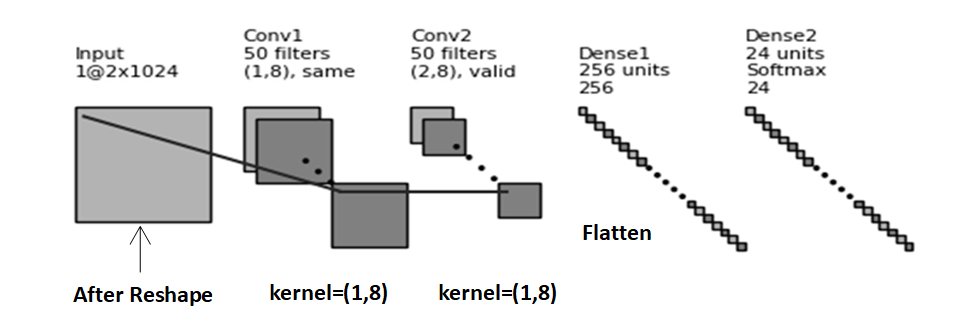
Figure 2. CNN architecture

The network uses two convolutional layers to extract the features of the input signal. There are not many convolutional layers and it is relatively lightweight. The extracted features are then passed through fully connected layers for classification. An Adam optimizer is employed, and dropout is applied after each convolutional layer for regularization, which helps to enhance the model's generalization capability. This architecture is well-suited for medium-scale radio frequency signal datasets and is commonly used in AMR tasks to handle various signal patterns.

2.3.3. Introduction to LSTM neural network and its advantages

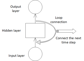
LSTM neural network originates from RNN. The biggest feature of RNN neural network is that the output of a neuron at a certain moment can be returned to the neuron as input, thereby maintaining the dependency relationship in the data [10]. Therefore, this series network structure is very suitable for the analysis of time series data. Figure 3 is an RNN network structure with a loop. Through the loop connection on the hidden layer, the network state at the previous moment can be passed to the current moment, and the state at the current moment can also be passed to the next moment [10].

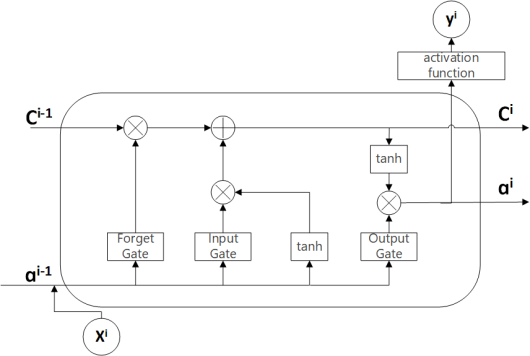
However, in practical applications, RNN has difficulty in preserving information for a long time due to problems such as gradient vanishing and gradient exploding [10]. Therefore, Hochreiter et al. proposed the LSTM neural network, which successfully overcomes the problems of gradient exploding in RNN and achieves accurate modeling of data with short-term or long-term dependencies [11]. The basic principle and working mode of LSTM are similar to those of RNN. Its core is to add a more refined internal unit memory cell to achieve the storage and update of information for the previous time and the next time. Figure 4 is a schematic diagram of the LSTM cell structure. The input gate determines which new information is added to the cell state, the forget gate determines which historical information needs to be discarded, and the output gate controls the contribution of the current cell state to the output. The memory cell (C) combines the input gate and the forget gate to update the cell state.

2.3.4. The CNN+LSTM hybrid neural network used in this research

From the above review, it is known that CNN neural networks are good at extracting local features of signals, and LSTM neural networks are able to capture the dependencies of signals through long and short-term memories, thus realizing the temporal dynamic modeling of neural networks. For modulated signals that are segmented and sampled by time, the introduction of LSTM can undoubtedly improve the recognition accuracy of the AMR task, especially for the lightweight CNN with only two convolutional layers used at the beginning of this paper. Therefore, this experiment adds a bidirectional LSTM layer on top of the initially used CNN code to capture long-term dependencies and dynamic changes in the signal, so that the model takes into account both pre- and post-textual information, making the modeling of the overall temporal characteristics of the signal more comprehensive and accurate. Figure 5 below shows the basic structure of this neural network:

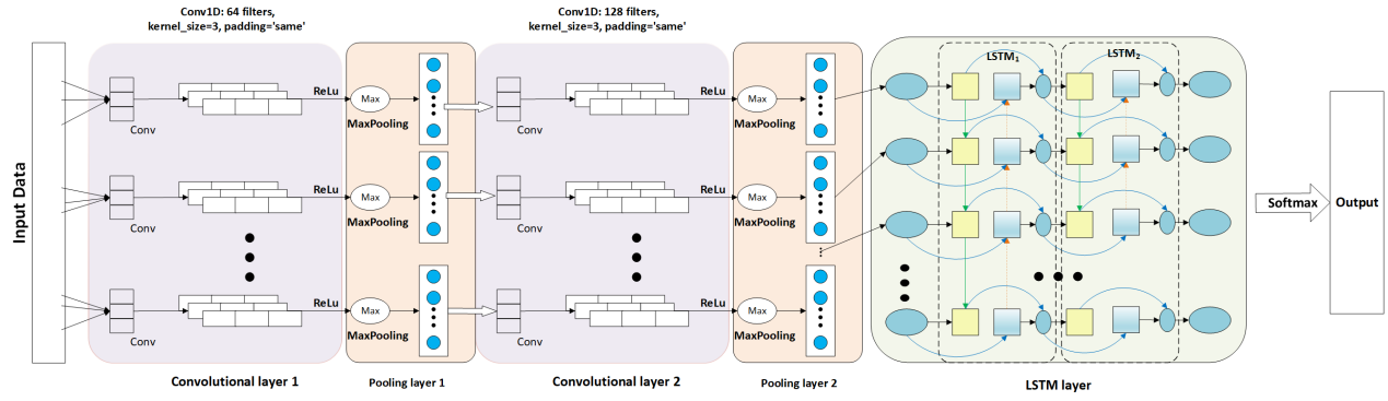
Figure 5. CNN_LSTM architecture

In the CNN part, the code first uses a Conv1D layer to extract primary features, and then preprocesses the data and reduces noise by batch normalization, pooling and dropout. Next, a deeper Conv1D layer is used to further extract complex features, and the same normalization and pooling are done to reduce the data dimensions to a size suitable for the LSTM layer input.

Then build two layers of bidirectional LSTM. The first layer returns the information of the entire sequence, allowing us to see the features of each time step; the second layer outputs the final summarized features. This allows us to capture the long-term dependencies in the signal. This enables the model to understand the global changes in the signal over time. Among them, the first layer of LSTM is set to 128 units, and return_sequences=True is set, so that each time step has an output, so that the subsequent layers can capture longer time series information. The second layer of LSTM also uses 128 units, but only returns the output of the last time step, thereby generating a compact global time series feature representation.

Finally, the time series features are integrated through the fully connected layer, and the Softmax layer is used to output the probability distribution of each modulation category. The entire structure fully combines the advantages of local feature extraction and time series dynamic modeling to achieve the purpose of improving the accuracy of automatic modulation recognition.

3. Experimental simulation

This experiment is based on Python 3.9 environment running under a Windows system, and the constructed neural network is trained and tested for recognition accuracy with the help of public datasets.

3.1. Dataset introduction and experimental settings

AMR methods based on Deep Learning are highly dependent on datasets. A comprehensive and high quality dataset is a key factor to support the development of DL-AMR, and its impact includes model training, testing and evaluation. The RML datasets1 are generated using GNU radio by O'Shea et al [9,12]. The RML2018.01a used in this paper was generated in a relatively good real laboratory environment. Table 1 is a description of the RML2018.01A dataset.

Table 1. RML2018.01a open datasets for SISO systems

Training 60% of the original dataset is used as the training set, 20% as the test set and 20% as the validation set. The neural network in this paper uses TensorFlow 2.1.0 as the Deep Learning framework, utilizing its seamless integration with Keras. The hardware of the experimental environment uses Intel(R) Core (TM) i9-12950HX CPU, 32G RAM and NVIDIA GeForce RTX 3070 Ti 8G memory graphics card.

The hyperparameter settings involved in the training process are shown in Table 2. As the training proceeds, the validation set loss will gradually decrease and the algorithm Patience=50 will be set. If the algorithm does not continue to converge and decrease for more than 50 iterations, the training will be terminated and the best trained model will be saved.

Table 2. Neural network parameter settings

In the experiments in this paper, the RML2018.01a dataset is partitioned into six different categories of Signal-to-Noise Ratio (SNR) conditions, namely 0db, 6db, 10db, 16db, 20db, and 30db. The noise at these six SNRs is sequentially from strong to weak, which more comprehensively covers the channel conditions in different environments from bad to excellent, and has the value of making practical use.

3.2. CNN Performance at Different SNRs

In the field of automatic modulation recognition, the confusion matrix is usually used to compare the difference between the predicted values and the true values. The confusion matrix results of the CNN model used in this paper under SNR of 0 dB, 6 dB, 10 dB, 16 dB, 20 dB, and 30 dB are shown in Figure 6 below.

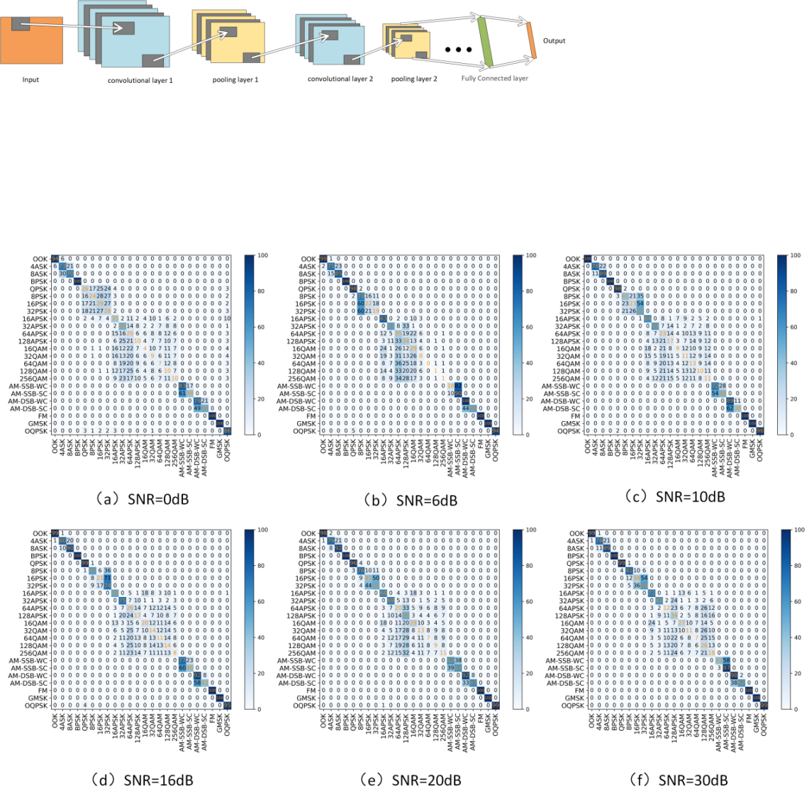
Figure 6. Confusion matrix of CNN model under different SNR

Meanwhile, for this CNN model, the automatic modulation recognition accuracy under the training set is shown in Table 3.

Table 3. Recognition accuracy of CNN model under 6 different SNRS

It can be seen that for this lightweight CNN neural network, even under excellent channel conditions with SNR>=20dB, its recognition accuracy is only about 60%, which is a very poor result. In a poor channel environment such as 0dB, the recognition accuracy is even lower than 50%, which basically can only recognize a few types of simple modulation modes, and basically can not do the recognition of high-order modulation modes such as 32QAM, 64QAM, 128QAM, and so on. The constellation points of these high-order modulation modes are distributed in the same orthogonal coordinate system, differing only in the number and density of constellation points. Noise, phase deviation or amplitude drift can cause the constellation point distribution areas to overlap. And these factors are difficult to distinguish for a lightweight, two-layer convolutional kernel CNN model.

3.3. CNN_LSTM performance at different SNRs

After introducing the LSTM neural network structure, the experimental confusion matrices at different SNRs are shown in Figure 7.

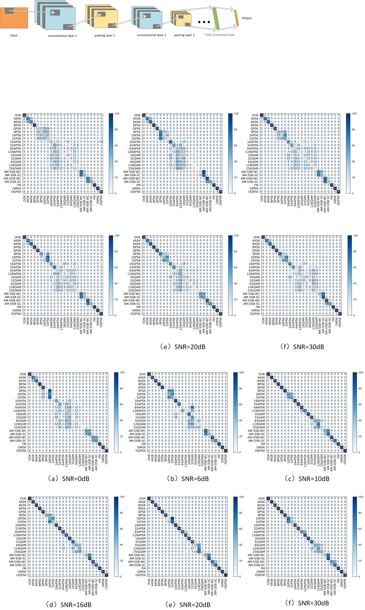
Figure 7. Confusion matrix of CNN_LSTM model under different SNR

For this CNN_LSTM model, the automatic modulation recognition accuracy under the data is shown in Table 4.

Table 4. Recognition accuracy of CNN_LSTM model under 6 different SNRS

The auto-tuning accuracy of the combined model is improved in all channel conditions compared to the single CNN network model. The recognition accuracy for good SNR conditions is greater than 80%, which is a significant improvement over the previously used CNN model. Also, the number of modulation types that this model has difficulty recognizing has been reduced, with only modulations such as higher-order QAM being difficult to recognize.

3.4. Results analysis

Through the previous experimental results, we know that the fused CNN+LSTM neural network introducing LSTM network structure improves the recognition accuracy significantly under the conditions of high SNR, which are all greater than 20%. The highest recognition rate of 85.6% is achieved at SNR=10dB, which is 29.9% higher than the single CNN model; while at low SNR, the combined model outputs are all more accurate than the traditional CNN model, with a recognition rate of 52.5% at SNR=0dB. This combined model enhances the noise-resistant performance of the recognition network in complex environments compared to the CNN model.

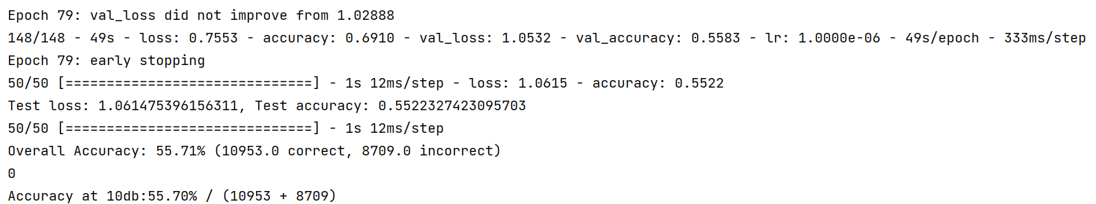
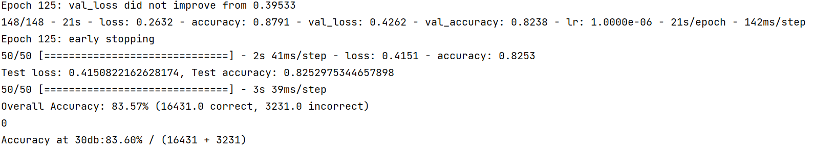
(a) CNN (b) CNN_LSTM

Figure 8. Each iteration time of different models in the experiment

In addition, from the running screenshot in Figure 8, it can be seen that the average iteration time per round of CNN network comes to 50s during the experiment, while the average iteration time per round of the combined CNN+LSTM network is only 20s. The reason is that the single CNN network will make the parameters of the subsequent fully-connected layer increase abruptly after Flatten due to the larger intermediate dimensionality graphs, which will increase the computation amount greatly and prolong the running time. In the hybrid model introducing LSTM, the sequence output of convolutional pooling followed by LSTM is usually more compact, and the dimension of Flatten is also smaller, thus only a relatively small fully connected layer is needed to complete the classification. This results in a hybrid model with fewer overall parameters and more efficient computation. In sequence learning, the temporal feature modeling of LSTM can partially replace the high-dimensional fully-connected layer, thus reducing the computational burden [13]. This greatly improves the experimental efficiency and is another advantage of combining neural networks.

4. Conclusion

In this paper, a lightweight CNN neural network model is reproduced, and then the network structure of LSTM neural network is introduced into the CNN model to form a hybrid model to improve the accuracy of automatic modulation recognition. Experimental comparisons show that the hybrid neural network model with CNN+LSTM structure combines the advantages of CNN local feature extraction and LSTM dynamic timing modeling, which is more effective in capturing the local and global features of the signal, and improves the recognition accuracy under various channel conditions. In addition, the hybrid model is more computationally efficient in each round of iteration due to the improved network structure during training, which shortens the overall training time and reduces the hardware requirements. The experimental results illustrate that the model outperforms some of the traditional methods on the RML2018.01A dataset, while verifying the importance of incorporating temporal modeling for automatic modulation recognition. However, there is still room for improvement, for example, higher-order modulations such as 64QAM, 128QAM and 256QAM in high SNR environments are still confusing. In conclusion, the CNN-LSTM hybrid model proposed in this paper improves the problem of low recognition accuracy of lightweight CNN model, and provides an efficient and highly robust solution for automatic modulation recognition, which has the potential for practical application.

References

[1]. Wang, C. X., You, X., Gao, X., Zhu, X., Li, Z., & Zhang, C. (2023). On the Road to 6G: Visions, Requirements, Key Technologies, and Testbeds. IEEE Communications Surveys & Tutorials, 25(2), 905-974.
[2]. Zhang, F., Luo, C., Xu, J., Luo, Y., & Zheng, F. C. (2022). Deep learning based automatic modulation recognition: Models, datasets, and challenges. Digital Signal Processing, 129, 103650.
[3]. Chen, H. (2025). Overview of Automatic Modulation Recognition Methods for Communication Signals Based on Deep Learning. Radio Engineering, 55(03), 526-539.
[4]. Nandi, T., & Nandi, A. (1993). Automatic digital modulation recognition using cumulants. IEEE Transactions on Communications, 41(8), 1092-1096.
[5]. Dobre, O. A., Abdi, A., Bar-Ness, Y., & Su, W. (2007). Survey of automatic modulation classification techniques: classical approaches and new trends. IET Communications, 1(2), 137-156.
[6]. Kulin, M., Kazaz, T., Moerman, I., et al. (2018). End-to-End Learning from Spectrum Data: A Deep Learning Approach for Wireless Signal Identification in Spectrum Monitoring Applications. IEEE Access, 6, 18484-18501.
[7]. Yao, Y., & Peng, H. (2019). Automation modulation recognition of the communication signals based on deep learning. Application of Electronic Technique, 45(2), 12-15.
[8]. Zhou, F. Y., Jin, L. P., & Dong, J. (2017). Review of Convolutional Neural Network. Chinese Journal of Computers, 40(06), 1229-1251.
[9]. O’Shea, T. J., Corgan, J., & Clancy, T. C. (2016). Convolutional radio modulation recognition networks. In C. Jayne & L. Iliadis (Eds.), Engineering applications of neural networks (pp. 213–226). Springer. https://doi.org/10.1007/978-3-319-44188-7_16
[10]. Yang, L. (2018). Research on recurrent neural network. Journal of Computer Applications, 38(S2), 1-6+26.
[11]. Hochreiter, S., & Schmidhuber, J. (1997). Long short-term memory. Neural Computation, 9(8), 1735-1780.
[12]. O’Shea, T. J., Roy, T., & Clancy, T. C. (2018). Over-the-air deep learning based radio signal classification. IEEE Journal of Selected Topics in Signal Processing, 12(1), 168-179.
[13]. Graves, A., Mohamed, A.-r., & Hinton, G. (2013). Speech recognition with deep recurrent neural networks. 2013 IEEE International Conference on Acoustics, Speech and Signal Processing (pp. 6645-6649). IEEE. https://doi.org/10.1109/ICASSP.2013.6638947
Cite this article
Jiang,Y. (2025). Deep Learning-based automatic modulation recognition: combination of CNN and LSTM neural network. Advances in Engineering Innovation,16(4),37-44.
Data availability
The datasets used and/or analyzed during the current study will be available from the authors upon reasonable request.
Disclaimer/Publisher's Note
The statements, opinions and data contained in all publications are solely those of the individual author(s) and contributor(s) and not of EWA Publishing and/or the editor(s). EWA Publishing and/or the editor(s) disclaim responsibility for any injury to people or property resulting from any ideas, methods, instructions or products referred to in the content.
About volume
Journal:Advances in Engineering Innovation
© 2024 by the author(s). Licensee EWA Publishing, Oxford, UK. This article is an open access article distributed under the terms and
conditions of the Creative Commons Attribution (CC BY) license. Authors who
publish this series agree to the following terms:
1. Authors retain copyright and grant the series right of first publication with the work simultaneously licensed under a Creative Commons
Attribution License that allows others to share the work with an acknowledgment of the work's authorship and initial publication in this
series.
2. Authors are able to enter into separate, additional contractual arrangements for the non-exclusive distribution of the series's published
version of the work (e.g., post it to an institutional repository or publish it in a book), with an acknowledgment of its initial
publication in this series.
3. Authors are permitted and encouraged to post their work online (e.g., in institutional repositories or on their website) prior to and
during the submission process, as it can lead to productive exchanges, as well as earlier and greater citation of published work (See
Open access policy for details).