1. Introduction

China is currently in a phase of high-quality economic development, with a rapid increase in the number of private cars. While a large number of private cars provide convenience for daily travel, they also bring enormous pressure to the transportation system. The congestion problem on urban roads is becoming increasingly severe, hindering normal travel and affecting the operational efficiency of cities, which in turn restricts social and economic development. Traffic flow prediction is one of the important means to address traffic congestion.

Traffic flow prediction can help people better plan travel routes and times, thereby saving time and economic costs. Transportation departments can understand the likelihood of congestion occurrence, quickly formulate optimal solutions, take timely measures such as adjusting traffic signal timing and dispatching traffic police for traffic guidance, thereby reducing the degree of road congestion and achieving more intelligent traffic management. Providing convenient and safe travel environment for citizens promotes the sustainable development of cities.

Early studies focused on temporal prediction, where traditional machine learning algorithms such as K-nearest neighbors [1] and SVR algorithms were widely used in the field of traffic prediction [2]. They have simple structures, are easy to understand, and implement. However, traditional machine learning methods have poor adaptability and often fail to fully capture the complex relationships in the data.

With the rapid development of artificial intelligence technology, more and more scholars are using deep learning methods [3-4]. Due to its excellent memory capability, recurrent neural networks (RNNs) [5] can learn long and short-term dependencies between sequence segments. However, during the computation process, problems such as gradient vanishing and exploding often occur. Using Long Short-Term Memory networks (LSTM) [6] for traffic flow prediction can address the problem of gradient vanishing or exploding that RNNs encounter when simulating long-term dependencies.

However, traffic flow in real life is influenced by both spatial and temporal factors. Spatial correlation is commonly present in traffic flow. Convolutional neural networks (CNNs) have shown significant effectiveness in dynamically extracting features from traffic data [7]. Since CNNs cannot effectively analyze non-Euclidean structured data and cannot efficiently explore the deep topological structures of graphs, introducing graph convolutional neural networks (GCNs) to handle graph-structured data in traffic prediction [8] can more accurately capture spatial dependencies in traffic data. The T-GCN [9] model utilizes GCN to capture spatial dependencies and GRU to capture temporal dependencies, modeling the spatiotemporal dependencies of traffic data. In fact, observations made at adjacent locations and times are not independent but dynamically correlated with each other. STGCN [10] adopts graph convolution to model spatial relationships in data and uses causal convolution to model temporal relationships. AGCRN [11] utilizes a node adaptive parameter learning module and a data adaptive graph generation module, combined with GRU networks, to achieve information transmission and updating. ASTGCN [12] proposes a novel spatiotemporal attention mechanism to capture spatiotemporal correlations, composed of spatial attention mechanism and temporal attention mechanism. A one-dimensional convolution is adopted at the temporal level, while GCN is adopted at the spatial level.

However, the above methods also have some issues. In representing the topological structure of traffic networks, fixed adjacency matrices are typically used, ignoring the spatial dynamic characteristics of traffic flow. Traditional graph convolutional neural networks tend to overly smooth during the convolution operation with increasing convolution layer depth. At this point, the aggregation radius of each node will reach a given threshold, and GCN may ignore the initial state of certain nodes. Traditional GCNs take the result of the last convolutional layer as output, and aggregating information from neighboring nodes only adds irrelevant information to each node, failing to effectively capture spatial correlations in traffic flow data.

Therefore, this paper proposes a model framework based on Adaptive Multi-channel Graph Convolutional Neural Networks for traffic flow prediction, which fully captures the spatiotemporal correlations in traffic flow data. By utilizing the method of adaptively learning adjacency matrices, embedding representations of nodes, and combining traffic flow data, the model adaptively learns adjacency matrices to capture dynamic relationships between nodes in complex traffic network structures. In the spatial dimension, a mixed skip propagation graph convolutional network model is employed, allowing it to retain the original node states and selectively obtain outputs of convolutional layers, thus avoiding the loss of node initial states and comprehensively capturing the spatial correlations of traffic flow.

2. Problem definition

Roads are abstracted as nodes, and the connection relationships between roads are abstracted as directed edges, forming a “node-edge” graph. The traffic road network is defined as a directed graph:

\( G=(V,E) \) (1)

Where, G represents the directed graph of the traffic road network; V is the set of road nodes; E is the set of directed edges.

The task of traffic flow prediction is to use historical traffic flow time data to predict future traffic flow data, which can be represented as:

\( [{X_{t+1}},...,{X_{t+T}}]=f(G;({X_{t-n}},...,{X_{t-1}},{X_{t}}))=(V,E) \) (2)

3. AMGCN model

In order to comprehensively explore and fully utilize the various spatiotemporal dependencies existing in the traffic network, this paper proposes a traffic flow prediction method based on Adaptive Multi-channel Graph Convolutional Neural Networks (AMGCN), integrating various attributes of traffic flow data for traffic flow prediction. The model utilizes an adaptive graph structure learning module to obtain graph structure information, which is then input into the graph convolution module to capture spatial dependencies. The temporal correlations of traffic flow data are captured through Long Short-Term Memory (LSTM) neural networks, resulting in the final output of the model. The structure of the model is illustrated in Figure 1.

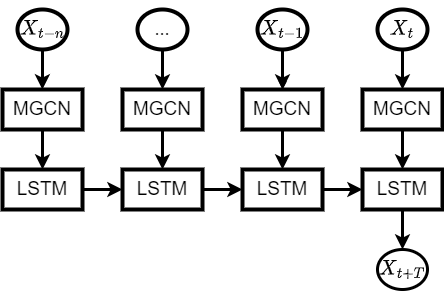
Figure 1. Structure of the AMGCN model

3.1. Adaptive graph learning module

The Adaptive Graph Learning Module dynamically learns graph structure information, enabling the model to adapt to the dynamic changes in traffic flow data and represent the directed relationships between nodes. Adaptive matrices are constructed through node embedding, where \( {E_{1}}ϵ{R^{N×d}} \) represents the original node embedding, \( {E_{2}}ϵ{R^{N×d}} \) represents the target node embedding, and the dimension of each node embedding is d. Then, similar to defining the graph through node similarity, the spatial dependency between each pair of nodes can be obtained by the inner product of embedding vectors \( {E_{1}} \) and \( {{E_{2}}^{T}} \) :

\( \hat{A}={I_{N}}+{D^{-\frac{1}{2}}}A{D^{-\frac{1}{2}}}={I_{N}}+SoftMax(RELU({E_{1}}∙{{E_{2}}^{T}})) \) (3)

Directly generating \( {D^{-\frac{1}{2}}}A{D^{-\frac{1}{2}}} \) instead of generating the adjacency matrix and calculating the Laplacian matrix helps avoid unnecessary resource wastage.

3.2. Spatial dimension graph convolution module

Traffic flow data exhibits complex spatial correlations. In order to analyze and extract the dynamic spatial characteristics of traffic flow, this paper proposes a Multi-Graph Convolutional Neural Network (MGCN) composed of mixed skip propagation layers. The purpose of the multi-graph module is to capture spatial dependencies in the traffic road network by integrating information from nodes and their neighboring nodes. The architecture of the mixed skip propagation layer is illustrated in Figure 2.

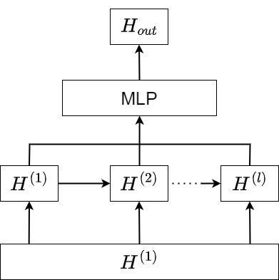
Figure 2. Structure of the MGCN

The MGCN mainly consists of two steps: information propagation and information selection.

First is information propagation. During this process, the information of each layer of nodes is collected from their neighboring nodes. Nodes update their own information based on the collected information, while filtering out irrelevant information to retain effective features, thereby reducing model complexity and improving computational efficiency. The computation for the l-th convolutional layer is as follows:

\( {H^{(l)}}=μ{H^{(1)}}+(1-μ)\hat{A}{H^{(l-1)}} \) (4)

where \( μ \) is a hyperparameter controlling the proportion of original node states, \( {H^{(l-1)}} \) represents the output of the \( l-1 \) -th layer, \( {H^{(l)}} \) represents the output of the \( l \) -th layer, and \( \hat{A} \) is the adaptive adjacency matrix.

After obtaining the outputs of all l convolutional layers, information aggregation is performed to retain the effective information generated at each skip. The definition of the information selection step is as follows:

\( {H_{out}}=\sum _{l=0}^{L}{H^{(l)}}{W^{(l)}} \) (5)

Where \( l \) is the number of layers of graph convolution, \( W \) represents the learnable parameter matrix, which serves as the feature selector.

3.3. LSTM module on the temporal dimension

Traffic flow exhibits temporal correlations, showing dynamic characteristics. Long Short-Term Memory (LSTM) neural networks avoid the problem of gradient explosion in recurrent neural networks and capture time dependencies by inputting traffic flow data with spatial features obtained from the graph convolution module into LSTM. The LSTM structure used in this paper is shown in Figure 3.

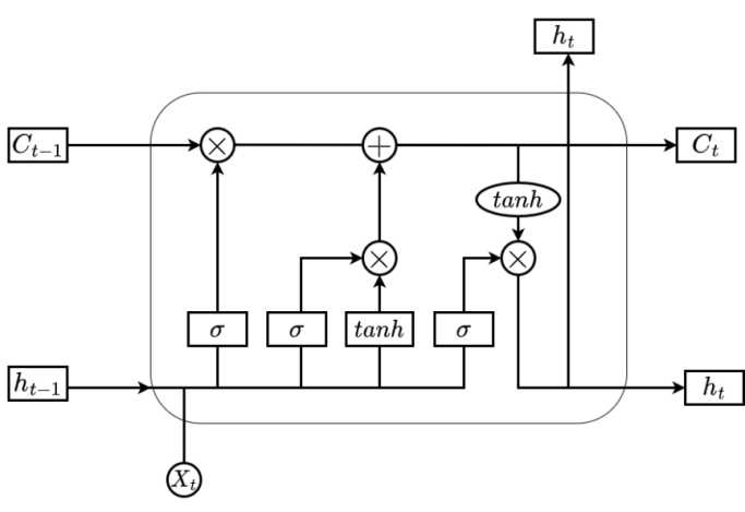
Figure 3. LSTM Structure

The computation is as follows:

\( \begin{cases}{f_{t}}=σ({W_{f}}∙[{h_{t-1}},h_{t}^{(l+1)}]+{b_{f}}) \\ {i_{t}}=σ({W_{i}}∙[{h_{t-1}},h_{t}^{(l+1)}]+{b_{i}}) \\ \widetilde{{C_{t}}}=tanh({W_{c}}∙[{h_{t-1}},h_{t}^{(l+1)}]+{b_{c}}) \\ tanh(x)=\frac{{e^{x}}-{e^{-x}}}{{e^{x}}+{e^{-x}}} \\ {C_{t}}={f_{t}}*{C_{t-1}}+{i_{t}}*\widetilde{{C_{t}}} \\ {o_{t}}=σ({W_{0}}∙[{h_{t-1}},h_{t}^{(l+1)}]+{b_{0}} \\ {h_{t}}={o_{t}}*tanh({C_{t}})\end{cases} \) (6)

Where: \( {i_{t}} \) represents the input gate, \( {f_{t}} \) represents the forget gate, \( {o_{t}} \) represents the output gate. \( h_{t}^{(l+1)} \) is the input at the current time, \( {h_{t-1}} \) is the state at the previous time step. The Sigmoid activation function is used to control the flow of information, selectively passing information. Its calculation results in a number between 0 and 1, achieving the selection and transmission of information in LSTM. The Sigmoid function is computed as follows:

\( σ(x)=\frac{1}{1+{e^{-x}}} \) (7)

3.4. Experimental setup and result analysis

3.4.1 Dataset introduction and data preprocessing

The dataset used in this section is collected by the Caltrans Performance Measurement System of the California Interstate Highway Network. This chapter predicts traffic flow data for the next hour using data from the past hour, where 12 data points constitute one time step. The dataset is split into training, validation, and testing sets in a ratio of 6:2:2, with the training set accounting for 60%, the validation set for 20%, and the testing set for 20%.

The detailed information of the dataset is shown in Table 1.

Table 1. Dataset Information

Perform z-score operation to normalize the data, aiming to enhance the convergence speed of the model:

\( {X^{ \prime }}=\frac{X-μ}{σ} \) (8)

Where \( X \) is the input data, \( μ \) is the mean of the data, and \( σ \) is the standard deviation.

To measure and evaluate the performance of different methods, three metrics are adopted: Mean Absolute Error (MAE), Mean Absolute Percentage Error (MAPE), and Root Mean Square Error (RMSE). Smaller values of these metrics indicate closer proximity between predicted and actual values, reflecting better predictive performance of the model. Conversely, larger values indicate poorer performance and greater deviation from the true samples.

(1) Mean Absolute Error (MAE):

\( MAE=\frac{1}{n}\sum _{i=1}^{n}|{Y_{i}}-{Y_{i}}| \) (9)

(2) Root Mean Square Error (RMSE):

\( RMSE=\sqrt[]{\frac{1}{n}\sum _{i=1}^{n}{({Y_{i}}-{\hat{Y}_{i}})^{2}}} \) (10)

(3) Mean Absolute Percentage Error (MAPE):

\( MAPE=\frac{100\%}{n}\sum _{i=1}^{n}|\frac{{Y_{i}}-{\hat{Y}_{i}}}{{Y_{i}}}| \) (11)

3.4.2 Benchmark models

The benchmark models used in this study are as follows:

VAR [13]: Vector Autoregressive model, which treats time series as a linear function to capture the time dependency of traffic flow data.

SVR [15]: Support Vector Regression model, which uses different kernel functions for regression and is suitable for predicting nonlinear relationship data.

LSTM [6]: Long Short-Term Memory network, consisting of three gates (forget gate, input gate, and output gate) used to capture time dependencies and widely applied in time series analysis.

DCRNN [15]: Diffusion Convolutional Recurrent Neural Network, which uses diffusion graph convolution layers to express topology and capture spatial dependencies, and utilizes RNN to encode temporal information.

STGCN [10]: Spatio-Temporal Graph Convolutional Networks, which uses spatial graph convolutional networks to capture spatial dependencies and one-dimensional convolution operation to extract temporal features.

Graph WaveNet [16]: This model introduces adaptive graphs to capture hidden spatial dependencies and utilizes dilated convolutions to capture temporal dependencies.

ASTGCN [12]: Spatial-Temporal Graph Convolutional Networks, which uses attention mechanisms to capture dynamic spatio-temporal relationships, where spatio-temporal convolutions are used to capture spatial patterns and temporal features.

AMGCN (ours): Adaptive Multi-channel Graph Convolutional Neural Networks model, which constructs the traffic network structure using adaptive adjacency matrices, captures spatial dependencies using MGCN, and captures temporal dependencies using LSTM.

3.4.3 Comparative analysis

Comparative analysis between the benchmark models and the proposed AMGCN model is conducted. The experimental results are shown in Table 2, indicating that the model proposed in this chapter performs well and outperforms the benchmark models on both datasets.

Table 2. Experimental Results

VAR, SVM, and LSTM are models used for time series prediction. However, traffic flow is a typical spatio-temporal data, and using these three methods for prediction cannot capture the spatial correlations between node data, leading to inaccurate predictions and large errors. DCRNN, STGCN, ASTGCN, Graph WaveNet, and the proposed AMGCN model all incorporate the representation of graph structure information and extract spatial features, resulting in higher prediction accuracy.

Comparative analysis reveals that the model proposed in this chapter outperforms other spatio-temporal models in terms of MAPE, MAE, and RMSE metrics. Traditional time series analysis methods exhibit large errors and low accuracy. The VAR model has the highest metrics, indicating low prediction accuracy. Based on linear assumptions, the VAR model’s simplistic structure cannot handle the non-linear relationships inherent in complex traffic flow data, making accurate modeling difficult. The LSTM model, based on deep learning methods, exhibits good performance in capturing long-term dependencies in time series. It effectively models complex data through its internal structure, relying on historical data for prediction and capturing time features. Therefore, its metrics are lower than VAR. However, both methods overlook the spatial correlations present in traffic flow data.

ASTGCN incorporates an attention mechanism while capturing temporal features by computing the influence weights between nodes to construct a dynamic traffic road map, thereby enhancing the model's predictive performance while considering the spatial correlations of traffic flow data. However, in the traffic road structure, there exist dynamic and complex relationships between nodes, and ASTGCN's prediction method does not exploit potential graph structural information. On the other hand, AMGCN learns hidden information between nodes through an adaptive graph structure learning module, automatically updating via gradient descent to capture dynamic node relationships, resulting in improved prediction results. As the traffic road graph structure changes with traffic road structures and traffic environments, AMGCN not only considers ordinary spatial distance dependencies but also constructs a new graph structure to better capture the spatial correlations of traffic flow and achieve better prediction results through the processes of information propagation and filtering.

4. Conclusion

This paper explores the learning mechanism of spatio-temporal correlations in traffic flow and proposes a prediction model based on a hybrid graph convolutional neural network to capture the spatio-temporal correlations of traffic flow, which is applied to traffic flow prediction tasks, demonstrating good performance. The AMGCN model utilizes adaptive adjacency matrices to model spatial road structures, combines MGCN and LSTM models to capture spatio-temporal correlations, and effectively predicts traffic flow at different road sections and time intervals, capturing the dynamic characteristics of traffic flow changes. Through training on the PeMS04 and PeMS08 datasets and conducting comparative experiments, the results indicate that AMGCN fully integrates the advantages of its components, effectively improving the accuracy of traffic flow prediction on road networks, demonstrating good predictive performance. In future work, collecting traffic flow data under different weather conditions, as well as data on accidents and traffic control sudden factors, to model the impact of external factors on traffic flow data, could lead to more accurate predictions.

References

[1]. Chang, H., Lee, Y., Yoon, B., & Baek, S. (2012). Dynamic near-term traffic flow prediction: systemoriented approach based on past experiences. Intelligent Transport Systems Iet, 6(3), p.292-305.
[2]. Zhao-Sheng, Y., Yuan, W., & Qing, G. (2006). Short-term traffic flow prediction method based on svm. Journal of Jilin University.
[3]. Fang, M., Tang, L., Yang, X., Chen, Y., & Li, Q. (2021). Ftpg: a fine-grained traffic prediction method with graph attention network using big trace data. IEEE Transactions on Intelligent Transportation Systems, PP(99), 1-13.
[4]. Yin, X., Wu, G., Wei, J., Shen, Y., Qi, H., & Yin, B. (2020). Deep learning on traffic prediction: methods, analysis and future directions.
[5]. Qu, L., Lyu, J., Li, W., Ma, D., & Fan, H. (2021). Features injected recurrent neural networks for short-term traffic speed prediction. Neurocomputing, 451, 290-304.
[6]. Hochreiter, S., & Schmidhuber, J. (1997). Long short-term memory. Neural Computation, 9(8), 1735-1780.
[7]. Méndez, M., Montero, C., Núñez, M. (2022). Using Deep Transformer Based Models to Predict Ozone Levels. In 14th Asian Conference on Intelligent Information and Database Systems, 169-182.
[8]. Wang, Y., Lv, Z., Sheng, Z., Sun, H., & Zhao, A. (2022). A deep spatio-temporal meta-learning model for urban traffic revitalization index prediction in the covid-19 pandemic. Advanced engineering informatics.
[9]. Zhao, L., Song, Y., Zhang, C., Liu, Y., & Li, H. (2019). T-GCN: a temporal graph convolutional network for traffic prediction.IEEE Transactions on Intelligent Transportation Systems, PP(99), 1-11.
[10]. Xiao, G., Wang, R., Zhang, C., & Ni, A. (2020). Demand prediction for a public bike sharing program based on spatio-temporal graph convolutional networks. Multimedia Tools and Applications(5).
[11]. Li, M., & Zhu, Z. (2021). Spatial-Temporal Fusion Graph Neural Networks for Traffic Flow Forecasting. National Conference on Artificial Intelligence.
[12]. Song, C., Lin, Y., Guo, S., & Wan, H. (2020). Spatial-Temporal Synchronous Graph Convolutional Networks: A New Framework for Spatial-Temporal Network Data Forecasting. (Vol.34, pp.914-921).
[13]. Hamilton, W. L., Ying, R., & Leskovec, J. (2017). Inductive representation learning on large graphs, 30: 1025-1035.
[14]. Gong, Jun, Qi, Lin, Liu, & Mingyue, et al. (2013). Forecasting urban traffic flow by SVR. Proceedings of the Chinese Control and Decision Conference, 981-984.
[15]. Li, Y., Yu, R., Shahabi, C., & Liu, Y. (2018). Diffusion Convolutional Recurrent Neural Network: Data-Driven Traffic Forecasting. International Conference on Learning Representations.
[16]. Wu, Z., Pan, S., Long, G., Jiang, J., & Zhang, C. (2019). Graph wavenet for deep spatial-temporal graph modeling, 1907-1913.
Cite this article
Xu,Z.;Gu,J. (2024). Research on traffic flow prediction method based on adaptive multi-channel graph convolutional neural networks. Advances in Engineering Innovation,7,41-47.
Data availability
The datasets used and/or analyzed during the current study will be available from the authors upon reasonable request.
Disclaimer/Publisher's Note
The statements, opinions and data contained in all publications are solely those of the individual author(s) and contributor(s) and not of EWA Publishing and/or the editor(s). EWA Publishing and/or the editor(s) disclaim responsibility for any injury to people or property resulting from any ideas, methods, instructions or products referred to in the content.
About volume
Journal:Advances in Engineering Innovation
© 2024 by the author(s). Licensee EWA Publishing, Oxford, UK. This article is an open access article distributed under the terms and
conditions of the Creative Commons Attribution (CC BY) license. Authors who
publish this series agree to the following terms:
1. Authors retain copyright and grant the series right of first publication with the work simultaneously licensed under a Creative Commons
Attribution License that allows others to share the work with an acknowledgment of the work's authorship and initial publication in this
series.
2. Authors are able to enter into separate, additional contractual arrangements for the non-exclusive distribution of the series's published
version of the work (e.g., post it to an institutional repository or publish it in a book), with an acknowledgment of its initial
publication in this series.
3. Authors are permitted and encouraged to post their work online (e.g., in institutional repositories or on their website) prior to and
during the submission process, as it can lead to productive exchanges, as well as earlier and greater citation of published work (See
Open access policy for details).