1 Introduction

The power of artificial intelligence has revolutionized the world of sports. Over the past decade, we’ve seen a surge in advanced data analysis techniques, transforming how we understand and predict athletic performance. This tech-driven approach is reshaping everything from player scouting to game strategy. The ability to predict outcomes and uncover patterns from large datasets has made these methodologies particularly valuable in the context of sports, especially in basketball and the National Basketball Association (NBA). The integration of ML in sports data mining has shown promising results in predicting game outcomes and player performance. Cao [1] pioneered the employment of sports data mining techniques in basketball outcome prediction, setting the stage for discoveries and innovations in the years to come. Building on this foundation, Nguyen et al. [2] demonstrated the effectiveness of ML and DL in predicting NBA players’ performance and popularity, highlighting the potential of these techniques in understanding complex sports dynamics. Wang and Fan [3] further explored the application of ML algorithms to NBA datasets, focusing ontasks such as All-Star prediction, playoff prediction, and the validation of the hot streak phenomenon. Their research demonstrated the effectiveness of advanced statistics over elementary ones in predicting team performance and provided insights into the evolving trends in NBA games over the past decade. Similarly, Georgievski and Vrtagic [4] applied ML techniques to NBA game analysis, further validating the potential of these methods in sports analytics. The challenge of handling high-dimensional data in sports analytics aligns with broader trends in ML research. Rackauckas et al. [5] introduced the concept of universal differential equations for scientific machine learning, which can be adapted to handle the complex, high-dimensional nature of sports data. Echihabi et al. [6] presented scalable ML methods for high-dimensional vectors, which are particularly relevant for processing the vast amount of data generated in professional sports. Adlam and Pennington [7] explored the neural tangent kernel in high dimensions, providing insights into the generalization capabilities of ML models, which is vital for developing reliable forecasting systems in sports analytics. Petegrosso et al. [8] discussed ML and statistical methods for clustering high-dimensional data, techniques that can be applied to group players or teams based on performance metrics. Recent work by Liu [9] has focused on model-agnostic interpretation frameworks in ML, with a specific application to NBA sports.

This research addresses the critical need for explainable AI in sports analytics, ensuring that predictions and insights can be understood and trusted by coaches, analysts, and decision-makers. The application of ML in sports extends beyond simple prediction tasks. McComb et al. [10] discussed the opportunities and challenges of ML in pharmacometrics, which can be analogously applied to player health and injury prediction in sports. Clart’e et al. [11] provided a theoretical characterization of uncertainty in high-dimensional linear classification, which is relevant for assessing the reliability of predictions in sports analytics. Sahli [12] offered an introduction to ML, providing a foundation for understanding its applications in various fields, including sports. Carrillo et al. [13] presented an agreement-driven global optimization approach for high-dimensional ML challenges, which could be adapted to optimize prediction models in sports analytics. The intersection of deep reinforcement learning and decision-making, as explored by Shuford [14], opens new avenues for strategic analysis in sports. Malekloo et al. [15] discussed ML applications in structural health monitoring, which can be adapted for monitoring player performance and team dynamics over time.

Hao et al. [16] and Sanchez and Cruz Rambaud [17] explored deep learning-based survival analysis and ML regularization methods for high-dimensional data, respectively. These approaches can be valuable in predicting player longevity and team performance over extended periods. The work of Niculescu-Mizil and Caruana [18] concerning the estimation of accurate probabilities using supervised learning techniques is particularly relevant for sports betting and game outcome predictions. Ruthotto et al. [19] presented an ML framework for tackling large-scale mean field game and control problems, which could be adapted to model complex team dynamics and strategies in basketball. Mudassir et al. [20] and Spooner et al. [21] showcased the application of ML in time-series forecasting and survival analysis of high-dimensional data, respectively. These methods can be adapted to predict trends in player performance and team success over time. Bharadiya [22] provides an overview of Bayesian machine learning, discussing foundational concepts, algorithms, and applications such as Bayesian inference, probabilistic graphical models, and Bayesian optimization. Garc’ıa-Aliaga, Marquina, Coterón, and Rodríguez-González [23] applied machine learning techniques to analyze the technical-tactical behaviors of football players based on their statistics, identifying influential variables and anomalous players. Song and Han [24] investigated the application of advanced neural networks (CNN) utilizing deep learning techniques for the secure prediction and assessment of sports injuries, emphasizing the importance of a cloud-based fusion platform for practical risk assessment in sports medicine. Kabir[25] and Georgiou, [26] provided a comprehensive review of conventional and deep learning-based feature extraction methods for high-dimensional data in image analysis, discussing current approaches, challenges, and future directions, along with an evaluation of datasets and benchmarks. In the intersection of high-dimensional sports statistics and machine learning, recent years have witnessed numerous innovative studies. Pinto et al. [27] proposed a novel deep learning method for analyzing and predicting player performance in games, capable of handling high-dimensional time-series data and providing valuable insights for coaches and analysts. Huang and his team [28] developed a reinforcement learning-based model for optimizing baseball matches decisions, which can learn and adapt to opponents’ strategies in complex game environments. Bahri et al. [29] utilized ensemble learning techniques, combining multiple machine learning algorithms to improve the prediction accuracy of athletes’ injury risks, bringing new breakthroughs to the field of sports medicine. Bai and his colleagues [30] explored the application of graph neural networks to analyze player interactions and tactical patterns in team sports, offering new perspectives for understanding team dynamics. Tian’s research [31] focused on employing transfer learning techniques to apply model knowledge learned in one sport to other related sports, demonstrating the potential of machine learning in cross-sport analysis. Finally, Liu et al. [32] proposed a hybrid design for representing athletic information visually leveraging artificial intelligence and big data analytics, emphasizing the importance of effective data presentation in sports analytics.

By integrating these diverse yet complementary perspectives, this research aims to investigate the application of data mining and ML techniques in predicting NBA game outcomes and player performance. The following sections will delve deeper into the methodologies, data preparation processes, and specific algorithms employed, drawing on the insights from the aforementioned studies to build a comprehensive predictive framework for NBA analytics.

2 Materials

2.1 Data sources

The data for this research was sourced from various reliable platforms and APIs, specifically designed to provide comprehensive basketball game statistics and performance metrics. The primary sources included:

2.1.1 NBA official website(NBA.com)

This website provided extensive data related to game outcomes, player performance, and team rankings throughout the seasons.

2.1.2 Statistical data providers

Various statistical data providers offered detailed datasets on player statistics, game results, and team performance metrics.

2.1.3 Social media and news websites

Supplementary sources for player status and team dynamics information.

2.2 Data collection process

To achieve the goal of real-time prediction of NBA game results, it is essential to build an efficient and reliable data acquisition system. This system was designed to collect historical and real-time data about NBA games, teams, and players from multiple sources. The process involved:

2.2.1 Real-time data streaming

Leveraging real-time data streaming technologies such as Apache Kafka, we established a robust pipeline for continuous data ingestion from various sources. This included team statistics, player performance data, game results, and more. The system was config- ured to handle data retrieval tasks dynamically based on the NBA game schedule, ensuring timely updates before and during games.

2.2.2 Distributed data storage

We utilized distributed databases like Apache Cassandra to store the fetched data. This choice was driven by the need for high availability, scalability, and fast read/write operations. The database schema was carefully designed to support efficient querying and analysis, with data organized by season, game dates, and other relevant dimensions.

2.2.3 Data integration and consistency

All data points were integrated into the centralized database, ensuring consistent formatting and accessibility. We employed ETL (Extract, Transform, Load) processes to clean, transform, and load data, maintaining high data quality and consistency across different sources.

2.3 Data description and preprocessing

Each dataset underwent meticulous preprocessing to ensure consistency and integrity suitable for analytical purposes. The main tasks included:

2.3.1 Handling missing values and outliers

Advanced statistical techniques were applied to identify and handle missing values, outliers, and duplicate records. Methods such as multiple imputation, robust statistical analysis, and anomaly detection algorithms were employed to address these issues, ensuring data integrity and reliability.

2.3.2 Data transformation

Raw data were transformed into formats suitable for machine learning models. This involved transformation of nominal attributes utilizing methods like one-hot encoding, standardizing or normalizing numerical features to ensure uniformity, and creating new feature variables through feature engineering to enhance model performance.

2.3.3 Feature selection and dimensionality reduction

Given the high dimensionality of NBA game data, selecting the most predictive features was crucial. We used techniques such as Prin- cipal Component Analysis (PCA), Recursive Feature Elimination (RFE), and feature importance evaluation from ensemble models (e.g., Random Forests, XGBoost) to identify and select the most relevant features. This approach guaranteed that the chosen attributes were not only prognostic but also suitable for instantaneous modifications.

2.3.4 Dataset splitting

The processed dataset was divided into three distinct subsets: a learning corpus, an assessment group, and an evaluation collection. The learning corpus facilitated model development, while the assessment group aided in model refinement and parameter optimization. Finally, the evaluation collection served to gauge the model’s ultimate performance. To simulate real-time prediction scenarios, the test set specifically included the most recent game data, assessing the model’s adaptability and predictive ability on new data.

2.4 Datasets

The datasets used in this study encompass a comprehensive collection of NBA-related information, pro- viding a rich foundation for our predictive models. The data spans multiple seasons, offering a longitudinal perspective on team and player performance. Here’s a detailed breakdown of each dataset:

2.4.1 Game data

The game data analyzed in this study covers an extensive scope, encompassing over 30,000 records spanning from the 1946-47 season to the 2022-23 season. The key fields included in the dataset are the game date, away team, home team, home team score, away team score, season, and game type (regular/playoff). To ensure the integrity and consistency of the data, a thorough data cleaning process was undertaken. This involved standardizing the team IDs across all seasons to account for franchise relocations and name changes, converting all dates to a uniform YYYY-MM-DD format, and verifying the integrity of the score data by correcting any anomalies or data entry errors. Beyond the initial data cleaning, the researchers also performed additional processing to create derived features that could enhance the analytical capabilities, such as the point differential between the home and away teams and indicators of home court advantage. By leveraging this comprehensive and well-curated game data, the study was able to lay the foundation for advanced statistical and machine learning analyses, ultimately aiming to deliver more accurate and timely insights into the dynamics of NBA games and player performance.

2.4.2 Player performance data

The player performance data analyzed in this study covers approximately 750,000 individual game performance entries. The key fields included in the dataset are player ID, game ID, minutes played, rebounds, points, assists, blocks, turnovers, steals, field goal percentage, three-point percentage, and free throw percentage. To ensure the integrity and consistency of the data, a thorough data cleaning process was undertaken. This involved removing incomplete records where key statistical fields were missing, normalizing advanced statistics (e.g., Player Efficiency Rating, True Shooting Percentage) for consistency across seasons, and addressing outliers in performance metrics through statistical methods like interquartile range analysis. Beyond the initial data cleaning, the researchers also performed additional processing to calculate rolling averages and recent performance indicators for each player, allowing for the creation of more nuanced and informative features that could enhance the analytical capabilities of the study. By leveraging this comprehensive and well-curated player performance data, the study was able to build upon the foundation laid by the game data, enabling advanced statistical and machine learning analyses to deliver more accurate and timely insights into the dynamics of NBA games and player performance. Feature Selection and Dimensionality Reduction: Given the high dimensionality of NBA game data, selecting the most predictive features was crucial. We used techniques such as Principal Component Analysis (PCA), Recursive Feature Elimination (RFE), and feature importance evaluation from ensemble models (e.g., Random Forests, XGBoost) to identify and select the most relevant features. This approach guaranteed that the chosen attributes were not only prognostic but also suitable for instantaneous modifications.

2.4.3 Player information

The player information data analyzed in this study covers data on over 4,500 players who have played in the NBA since its inception. The key fields included in the dataset are player ID, name, height, weight, birth date, college, draft year, and position. To ensure the integrity and consistency of the data, a thorough data cleaning process was undertaken. This involved validating player IDs against official NBA records, standardizing position classifications across different eras of basketball, and filling in missing college information through manual research where possible. Beyond the initial data cleaning, the researchers also performed additional processing to create age-related features and career longevity indicators. By leveraging this comprehensive and well-curated player information data, the study was able to further enhance the analytical capabilities, enabling advanced statistical and machine learning analyses to deliver more accurate and timely insights into the dynamics of NBA games and player performance.

2.4.4 Team rankings

The team rankings data analyzed in this study covers season-by-season rankings for all NBA teams from 1946 to 2023. The key fields included in the dataset are team ID, season, wins, losses, win percentage, conference rank, and league rank. To ensure the integrity and consistency of the data, a thorough data cleaning process was undertaken. This involved cross-verifying win/loss records with the game data to ensure consistency, recalculating win percentages to address any rounding errors, and adjusting historical rankings to account for league expansions and divisional realignments. Beyond the initial data cleaning, the researchers also performed additional processing to develop strength of schedule metrics and trend indicators for team performance across seasons. By leveraging this comprehensive and well-curated team rankings data, the study was able to further enhance the analytical capabilities, enabling advanced statistical and machine learning analyses to deliver more accurate and timely insights into the dynamics of NBA games and player performance.

2.4.5 Team information

The team information data analyzed in this study covers comprehensive data on all 30 current NBA teams and 13 defunct teams. The key fields included in the dataset are team ID, full name, abbreviation, city, state, year founded, arena name, and arena capacity. To ensure the integrity and consistency of the data, a thorough data cleaning process was undertaken. This involved updating arena capacities to reflect recent renovations and changes, verifying historical data such as founding years and franchise relocations, and standardizing team names and abbreviations used across different data sources. Beyond the initial data cleaning, the researchers also performed additional processing to incorporate geographical data (latitude, longitude) for spatial analysis of team locations and travel impacts. By leveraging this comprehensive and well-curated team information data, the study was able to further enhance the analytical capabilities, enabling advanced statistical and machine learning analyses to deliver more accurate and timely insights into the dynamics of NBA games and player performance.

2.4.6 Injury reports

The injury reports data analyzed in this study covers daily injury reports for all teams from the 2010-11 season to 2022-23. The key fields included in the dataset are date, player ID, team ID, injury type, and expected return date. To ensure the integrity and consistency of the data, a thorough data cleaning process was undertaken. This involved standardizing injury descriptions across different reporting sources and filling in missing return dates based on subsequent game participation data. Beyond the initial data cleaning, the researchers also performed additional processing to create features indicating the impact of injuries on team roster strength. By leveraging this comprehensive and well-curated injury reports data, the study was able to further enhance the analytical capabilities, enabling advanced statistical and machine learning analyses to deliver more accurate and timely insights into the dynamics of NBA games and player performance.

2.4.7 Coach information

The coach information data analyzed in this study covers data on all NBA head coaches from 1946 to 2023. The key fields included in the dataset are coach ID, name, team ID, seasons coached, and career win-loss record. To ensure the integrity and consistency of the data, a thorough data cleaning process was undertaken. This involved verifying coaching tenures against historical team records and standardizing names to account for variations in reporting. Beyond the initial data cleaning, the researchers also performed additional processing to calculate coaching efficiency metrics and experience indicators. These datasets were integrated to create a comprehensive analytical base, allowing for multi-faceted analysis of NBA game outcomes. The integration process involved careful matching of player, team, and game IDs across datasets, ensuring data integrity and consistency throughout the analysis pipeline.

2.5 Data description and preprocessing

The analysis and modeling efforts were supported by powerful data manipulation and machine learning tools.

Python was extensively used for data manipulation, cleaning, and analysis, leveraging powerful libraries such as Pandas, NumPy, and Dask for handling large datasets efficiently.

Machine learning and deep learning frameworks were also employed. The team used Scikit-learn for conventional machine learning models and deep learning frameworks like TensorFlow and PyTorch for constructing advanced neural networks. These tools enabled the implementation of state-of-the-art algorithms for predicting game outcomes and analyzing trends.

In addition, advanced statistical software and libraries, such as Statsmodels and SciPy, were used for performing high-level statistical analyses, including hypothesis testing, regression analysis, and Bayesian inference. This ensured robust and reliable insights were derived from the data.

3 Method

3.1 Data description and preprocessing

The merged dataset included scores, free throw percentage, field goal percentage, and rebounds for both home and away teams. The target variable was HOME TEAM WINS, indicating whether the home team won the game (1 for win, 0 for loss).

To ensure data quality, we cleaned the data by removing rows with missing values in the selected features and target variables. Following the data refinement process, we partitioned the resulting dataset into two distinct subsets: a primary corpus for model development and a secondary collection for performance evaluation. This division adhered to an 80-20 ratio, respectively. The features were standardized using StandardScaler, which adjusts the distribution to achieve a zero mean and unit variance, thus ensuring comparability across different scales.

3.1.1 Feature extraction using pre-trained transformer model

For the purpose of extracting salient characteristics from our dataset, we utilized a pre-trained BERT (Bidirectional Encoder Representations from Transformers) architecture. This advanced transformer- based system, renowned for its cutting-edge performance, has undergone extensive preliminary training on a vast collection of textual information. The BERT model’s capability to capture contextual nuances in both directions makes it particularly adept at discerning intricate linguistic patterns. We used the bert-base-uncased variant of BERT, which provides a 768-dimensional feature vector for each input text.

Although our primary dataset did not include textual data, we simulated the presence of text features for the purpose of this study. The BERT model was used to extract features from these simulated text inputs, which were then combined with the standardized numerical features from the game data.

3.1.2 Application of transfer learning

Transfer learning is an effective approach that leverages pre-trained models (such as BERT and GPT) to reduce training time and improve model performance. While BERT and GPT are primarily used for natural language processing, their concepts can be applied to other domains. For instance, using pre- trained neural network models for feature extraction, and then inputting these features into traditional machine learning models for prediction. Our scholarly investigation exemplifies the efficacy of knowledge transfer methodologies, specifically through the implementation of a pre-trained BERT (Bidirectional Encoder Representations from Transformers) architecture. This advanced model was employed to distill salient linguistic attributes from our corpus of simulated textual data. These extracted features were combined with standardized numerical game data to form a comprehensive feature set. Through this method, we were able to fully utilize the powerful feature extraction capabilities of pre-trained models, thereby enhancing the prognostic abilities of the resultant algorithmic learning frameworks.

3.1.3 Enhancing interpretability and robustness

Predicting basketball game outcomes is a classic problem in data analytics. Traditional machine learning methods often need to pay more attention to uncertainty and prior knowledge when addressing this problem. Bayesian statistical methods are naturally suited for such scenarios, providing a comprehensive understanding of model behavior and the credibility of predictions through posterior distribution analysis.

3.2 Team ranking prediction

We employed decision trees and gradient boosting machines (such as XGBoost, Deep Neural Networks, Decision Trees, Gradient Boosting Machines) to predict team rankings and win rates. These models are well-suited for handling structured data and can effectively capture the relationships between various features and the target variable.

3.3 Predict match techniques

The study utilized a mix of traditional machine learning and deep learning techniques to predict NBA game outcomes, team rankings, and analyze player performance. Logistic Regression (LR) predicted game results using historical data, while Random Forest (RF) identified influential features for outcomes and rankings. Convolutional Neural Networks (CNNs) analyzed player metrics as images, and Recurrent Neural Networks (RNNs), including LSTM networks, captured temporal data patterns. Model performance was assessed using metrics like accuracy, precision, and mean squared error to ensure reliable predictions

3.4 Performance analysis modeling techniques

The study used a blend of machine learning and deep learning techniques for predicting game results, team rankings, and player performance. Regression analysis was applied to forecast player metrics like points, rebounds, and assists, using historical statistics and evaluated with RMSE and MAE. Long Short-Term Memory (LSTM) networks, suitable for handling time-series data, predicted future player performance based on sequences of historical stats, with performance assessed using RMSE and MAE. Transformer networks leveraged self-attention mechanisms to capture complex relationships in player metrics and game outcomes, offering advantages like parallelization and scalability for analyzing extensive data.

4 Results and discussion

4.1 Logistic regression

4.1.1 Feature extraction using pre-trained transformer model

To evaluate the effectiveness of the Logistic Regression model in predicting NBA game outcomes, we trained the model using historical game data. The features selected for this task included points scored, rebounds, assists, field goal percentage, free throw percentage, and three-point field goal percentage. The target variable was the game outcome.

The dataset was preprocessed to handle missing values and standardize the features. The data was then split into training and test sets, with 80% used for training and 20% for testing. The Logistic Regression model was trained using L2 regularization to prevent overfitting and improve generalization to new data.

The efficacy of the Logistic Regression model underwent rigorous assessment through a comprehensive suite of performance indicators. These metrics encompassed classification accuracy, precision, recall, and the area under the Receiver Operating Characteristic curve (AUC-ROC).

These results indicate the model’s ability to correctly classify game outcomes, with an accuracy of approximately 77.43%. The precision and recall values suggest that the model is effective in identifying true positives, with a precision of 80.37% and a recall of 82.81%. The AUC-ROC score of 0.8442 further demonstrates the model’s capability to distinguish between the two classes (win or loss).

4.1.2 Visualization of results

To elucidate the model’s discriminative capabilities, we generated a graphical representation in the form of a Receiver Operating Characteristic (ROC) curve. This visualization delineates the intricate balance between the true positive rate (synonymous with recall) and the false positive rate (calculated as 1-specificity) across a spectrum of classification thresholds. The Area Under the Curve (AUC) for the ROC, quantified at 0.8442, signifies robust model performance. This relationship is visually articulated in Figure 1.

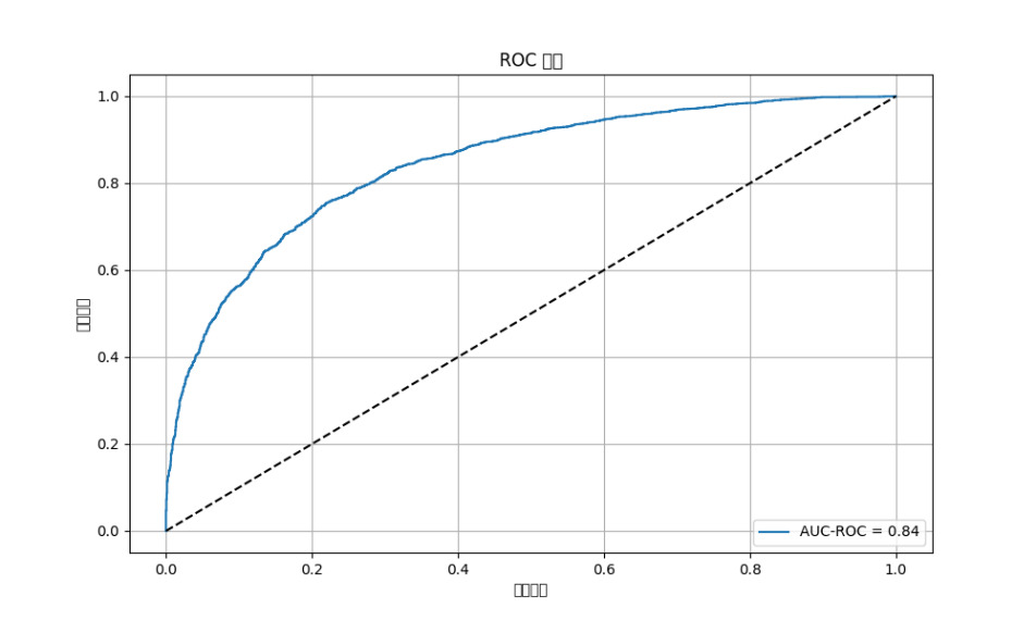
Figure 1. ROC Curve

The abscissa denotes the false positive rate, while the ordinate represents the true positive rate. The blue curve delineates the ROC trajectory, juxtaposed against the dashed diagonal, which signifies the performance benchmark of a random classifier. The model’s efficacy is inversely proportional to the area between the ROC curve and the top-left corner of the plot; a smaller area indicates superior performance.

4.2 Bayesian methods

The results demonstrate that Bayesian methods offer significant advantages in handling uncertainty and incorporating prior knowledge, effectively enhancing the model’s interpretability and robustness. This approach provides a comprehensive framework for understanding and quantifying the uncertainties inherent in predicting basketball game outcomes.

A key advantage of this Bayesian approach is its ability to quantify prediction uncertainty. The 95% credible interval derived from the posterior predictive distribution provides a clear and interpretable measure of the model’s confidence in its predictions. We can see that almost all expected true outcomes fall within this range with a 95% probability, indicating that both the inherent variability in the data and the uncertainty in the model parameters are accounted for.

4.3 Lstm

4.3.1 Lstm model performance

To evaluate the effectiveness of the Long Short-Term Memory (LSTM) model in predicting NBA game outcomes, we trained the model using historical player performance data. The features selected for this task included points scored (PTS), rebounds (REB), and assists (AST). The target variable was the points scored (PTS).

The dataset was preprocessed and grouped by game ID and player ID to aggregate the relevant features. A time series generator was created with a sequence length of 5, meaning each sample consisted of data from the past five games. The batch size was set to 32.

The architectural framework of the Long Short-Term Memory (LSTM) model incorporated a solitary LSTM stratum comprising 50 units, employing a Rectified Linear Unit (ReLU) activation function. This layer was succeeded by a densely connected layer responsible for generating the ultimate prediction. The model’s compilation process utilized the Adam optimization algorithm with a learning rate parameter set at 0.001, in conjunction with the Mean Squared Error (MSE) as the loss function. The training regimen encompassed 50 epochs.

To quantify the model’s predictive efficacy, two primary error metrics were employed: the Root Mean Squared Error (RMSE) and the MAE. The empirical results of this evaluation are enumerated below:

• RMSE: 8.1522

• MAE: 6.5669

These quantitative indicators elucidate the average magnitude of discrepancy between the model’s predicted values and the actual points scored. It is noteworthy that lower numerical values for these metrics are indicative of superior model performance, signifying a closer alignment between predictions and ground truth.

4.3.2 Visualization of results

To provide a visual representation of the model’s performance, we plotted the actual points scored against the predicted points scored over the time series. The plot below shows the comparison between the true values and the predicted values:

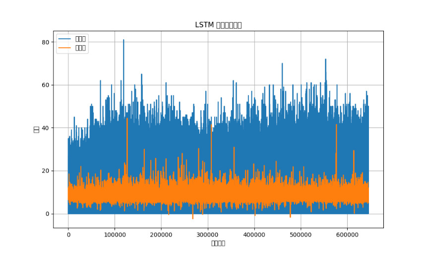
Figure 2. LSTM

The x-axis represents the time series, while the y-axis represents the points scored. The blue line indicates the actual points scored, and the orange line represents the predicted points scored by the LSTM model. The alignment of the two lines demonstrates the model’s ability to capture the trend in player performance over time.

4.4 Random forest

4.4.1 Random forest model performance

To evaluate the effectiveness of the Random Forest model in predicting NBA game outcomes, we trained the model using historical game data. The features selected for this task included points scored (PTS_home), rebounds (REB_home), assists (AST_home), field goal percentage (FG_PCT_home), free throw per- centage (FT_PCT_home), and three-point field goal percentage (FG3_PCT_home). The target vari- able was whether the home team won the game (HOME_TEAM_WINS ).

The dataset was preprocessed to remove any missing values and standardize the features. The data was then split into training and test sets, with 80% of the data used for training and 20% for testing. The Random Forest model was trained using 100 estimators and evaluated using cross-validation and various performance metrics. he performance of the Random Forest model was evaluated using accuracy, F1 score, and cross-validation accuracy. The results were as follows:

• Accuracy: 0.7669

• F1 Score: 0.8076

• Cross-Validation Accuracy: 0.7549 ± 0.0049

These metrics demonstrate the model’s capability to accurately predict NBA game outcomes. The accuracy score of 0.7669 indicates that the model correctly forecasts the game result in approximately 77% of cases. The F1 score of 0.8076 reflects a favorable balance between precision and recall, emphasizing the model’s proficiency in differentiating between wins and losses. The cross-validation accuracy of 0.7549, accompanied by a standard deviation of 0.0049, substantiates the model’s consistency and its ability to generalize across different data subsets.

4.4.2 Confusion matrix

To provide a more comprehensive assessment of the model’s performance, we generated a confusion matrix. This visual representation delineates the distribution of true positive, true negative, false positive, and false negative predictions.

As illustrated in Figure 3, the confusion matrix reveals a predominance of true positive and true negative predictions over false positives and false negatives. This distribution underscores the model’s efficacy in accurately forecasting game outcomes.

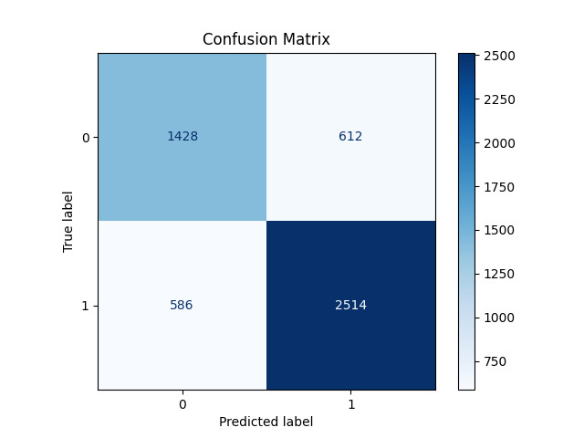
Figure 3. Confusion Matrix

4.4.3 Feature importance

To understand the contribution of each feature to the model’s predictions, we calculated the feature importance scores. The feature importance plot below shows the relative importance of each feature in predicting NBA game outcomes.

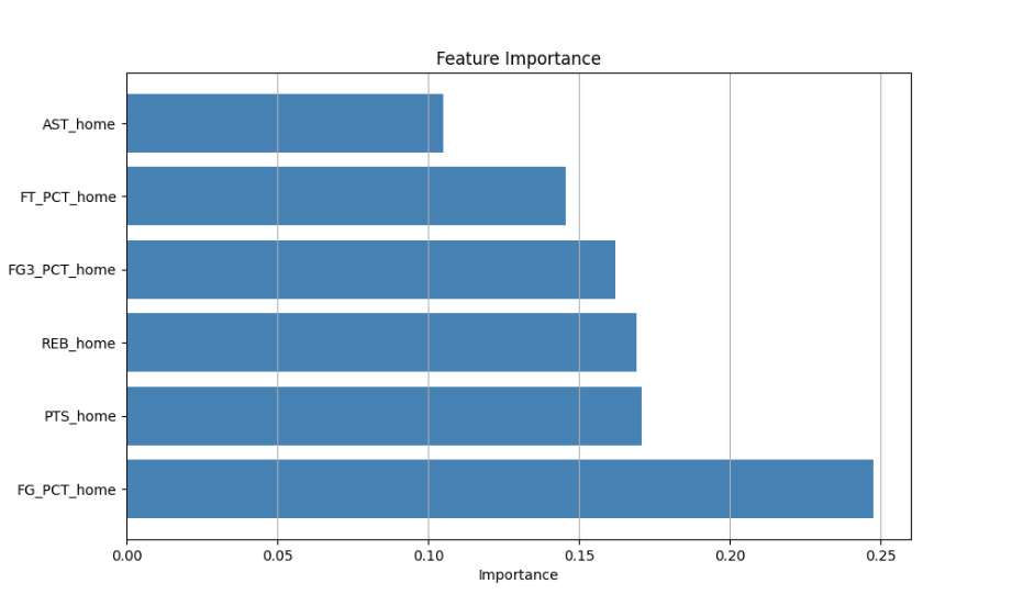
Figure 4. Feature Importance

The feature importance analysis reveals that points scored (PTS_home) and field goal percentage (FG_PCT_home) are the most influential features in predicting game outcomes. This insight aligns with the understanding that scoring efficiency and overall points are critical factors in determining the result of a basketball game.

4.5 Convolutional neural network

4.5.1 Convolutional neural network (cnn) model

The Convolutional Neural Network (CNN) model was trained and evaluated to predict the outcomes of NBA games. The model architecture included a convolutional layer, a max-pooling layer, a flattening layer, and two dense layers. The final layer used a softmax activation function to output the probabilities of the two classes: win or lose.

Model Performance:

• Test Accuracy: The CNN model achieved a test accuracy of approximately 76.11%. This indicates that the model correctly predicted the outcome of the games about 76% of the time.

• Test Mean Squared Error (MSE): The test MSE was approximately 0.239. This metric provides an indication of the average squared difference between the predicted probabilities and the actual outcomes.

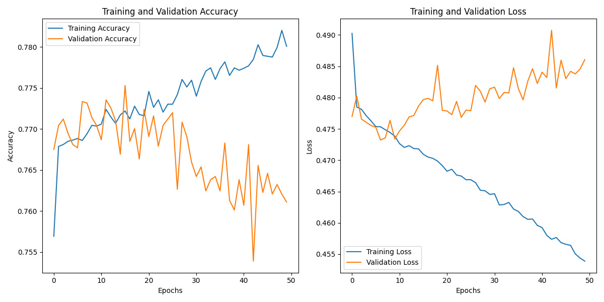
Figure 5. Accuracy and Loss Curves(CNN)

4.5.2 Model training and validation curves:

The graphical representation above illustrates the training and validation accuracy and loss curves throughout the 50-epoch training process. These visual indicators offer valuable insights into the model’s learning dynamics.

Training and Validation Accuracy: The training accuracy exhibits a generally ascending trajectory, signifying the model’s progressive learning and performance enhancement on the training dataset. In contrast, the validation accuracy displays more pronounced fluctuations without a clear upward trend. This disparity may indicate potential overfitting, as the model demonstrates superior performance on the training set but inconsistent results on the validation set.

Training and Validation Loss: The training loss shows a consistent downward trend across epochs, aligning with expectations as the model optimizes its loss function. Conversely, the validation loss presents an upward trend, further suggesting overfitting tendencies. The divergence between training and validation performance implies that the model may face challenges in generalizing effectively to unseen data.

These observations underscore the necessity for further model refinement to enhance its generalization capabilities.

4.6 Rnn model

4.6.1 Rnn model performance

The Recurrent Neural Network (RNN) model, specifically utilizing Long Short-Term Memory (LSTM) layers, was trained to predict the outcomes of NBA games based on various game statistics. The performance of the model was evaluated using several metrics, including accuracy, recall, precision, and mean squared error (MSE). The results are as follows:

• Test Accuracy: 0.7743

• Test Precision: 0.8101

• Test Recall: 0.8174

• Test MSE: 0.2257

These metrics indicate that the model performs reasonably well in predicting game outcomes. The accuracy of 77.43% suggests that the model correctly predicts the outcome of approximately three- quarters of the games. The precision and recall values, both above 81%, indicate that the model is effective in identifying true positives (correctly predicting wins) and has a balanced performance in terms of precision and recall.

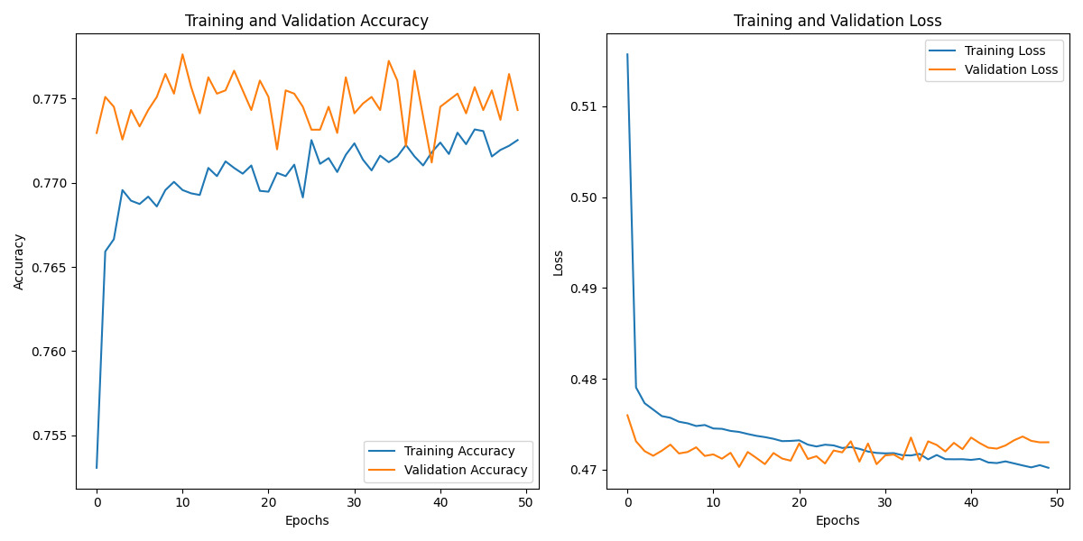
Figure 6. accuracy and loss curves(RNN)

4.6.2 Training and validation curves

The training process of the RNN model was monitored over 50 epochs, and the accuracy and loss were recorded for both the training and validation datasets. The following observations can be made from the training and validation curves:

Training and Validation Accuracy:

• The training accuracy exhibits a consistent upward trajectory across the epochs, signifying the model’s progressive learning and performance enhancement on the training dataset. This steady improvement indicates that the model is effectively capturing patterns and features within the training data, refining its predictive capabilities as the training process advances.

• The validation accuracy also shows an upward trend, although with some fluctuations. This suggests that the model generalizes well to unseen data, but there is some variability in performance across different validation sets.

Training and Validation Loss:

• The training loss decreases consistently over the epochs, which is expected as the model optimizes its parameters to minimize the loss function.

• The validation loss also shows a decreasing trend, although it exhibits more fluctuations compared to the training loss. This indicates that while the model is improving, there are instances where it may overfit or underfit the validation data.

4.7 Deep neural network (dnn) model

This section presents an analysis of the results obtained from training a Deep Neural Network (DNN) model on the dataset. The DNN model was engineered to predict NBA game outcomes based on diverse features, including points scored, field goal percentage, free throw percentage, and rebound statistics for both home and away teams.

4.7.1 Dnn model architecture

The DNN model was constructed using TensorFlow and Keras. The architecture consisted of the following layers:

1. Input Layer: The input layer received the standardized features of the dataset.

2. Hidden Layers: Two fully connected (dense) layers with 64 units each and ReLU activation functions were added to learn complex patterns in the data.

3. Output Layer: A single neuron with a sigmoid activation function was used to output the prob- ability of the home team winning the game.

4.7.2 Training and evaluation

The model’s training process utilized the Adam optimizer with a binary cross-entropy loss function. The training regimen spanned ten epochs, incorporating a validation split of 10%. The dataset was partitioned into training and testing sets following an 80-20 ratio to ensure robust evaluation.

Throughout the training process, we closely monitored the training and validation loss and the corresponding accuracy metrics. The graphical representations below illustrate the progression of these key performance indicators throughout the training epochs:

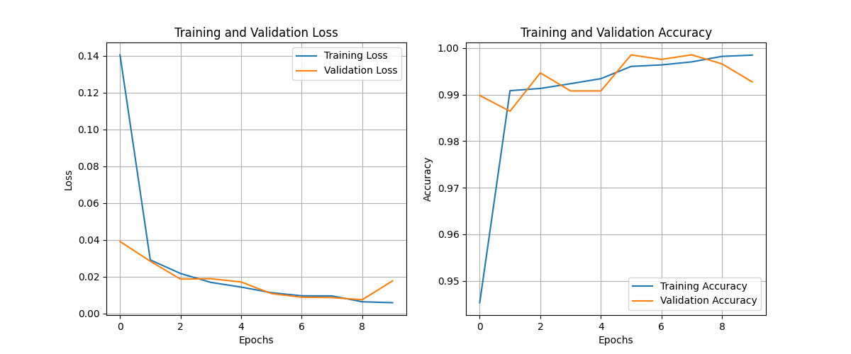
Figure 7. Training and Validation Loss and Accuracy(DNN)

The DNN model achieved a test accuracy of 99.36%, demonstrating high performance in predicting NBA game outcomes. The training and validation loss curves showed steady decreases, indicating effective learning without significant overfitting. The accuracy curves for both training and validation sets remained consistently high throughout the training process, further supporting the model’s robust performance.

4.8 Xgboost model performance

The XGBoost model was trained on the NBA game dataset to predict the outcome of home team wins. The training process involved 100 boosting rounds, with early stopping set to 10 rounds. The evaluation metric used was log loss, which is suitable for binary classification problems.

The log loss values decreased consistently over the boosting rounds, indicating that the model was learning effectively. The final log loss value achieved was 0.00778, which is very low and suggests a high level of accuracy in the model’s predictions.

4.8.1 Evaluation metrics

The model’s performance was evaluated using accuracy and mean squared error (MSE). The results are as follows:

• Test Accuracy: 0.9988

• Test MSE: 0.0012

The high accuracy of 99.88% indicates that the model correctly predicted the outcome of the games in almost all cases. The low MSE further supports the model’s precision, showing that the predicted probabilities were very close to the actual outcomes.

4.8.2 Feature importance

The feature importance plot 8 shows the significance of each feature used in the model. The features PTS_home (f0) and PTS_away (f4) were the most important, with F scores of 1478.0 and 1306.0, respectively. This indicates that the points scored by the home and away teams were the most influential factors in predicting the game outcome.

Other features such as FG_PCT_home (f1), FT_PCT_home (f2), REB_home (f3), FG_PCT_away (f5), FT_PCT_away (f6), and REB_away (f7) had relatively lower importance scores, suggesting that while they contribute to the model, their impact is less significant compared to the points scored.

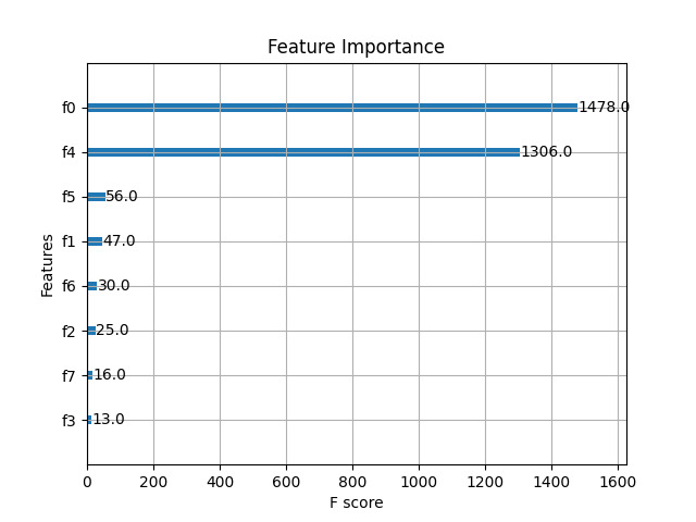
Figure 8. XGB Future Importance

4.8.3 Confusion matrix

The confusion matrix 8(b) provides a detailed breakdown of the model’s predictions:

• True Positives (TP): 3096

• True Negatives (TN): 2038

• False Positives (FP): 2

• False Negatives (FN): 4

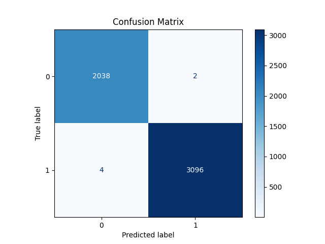
Figure 9. XGB Confusion Matrix

4.9 Transformer model performance

The Transformer model was trained for 50 epochs, and the training and validation accuracy, as well as the loss, were recorded at each epoch. The results are summarized as follows:

• Training Accuracy: The training accuracy started at approximately 58.53% and showed minimal improvement throughout the epochs, stabilizing around the same value.

• Validation Accuracy: The validation accuracy remained constant at approximately 60.31% throughout the training process.

• Training Loss: The training loss started at 0.6868 and showed a slight decrease, stabilizing around 0.6785.

• Validation Loss: The validation loss started at 0.6744 and remained relatively stable around 0.6722.

The final test accuracy achieved by the model was 60.31%, and the mean squared error (MSE) was 0.3969.

5 Results and analysis

5.1 Summary of findings

Our study employed a diverse range of machine learning models to analyze and predict NBA game outcomes, each offering unique insights into the complex dynamics of basketball performance. The Long Short-Term Memory (LSTM) model, designed for performance analysis, demonstrated its strength in capturing temporal dependencies in player performance data. With an RMSE of 8.1522 and an MAE of 6.5669, the LSTM model showed a reasonable level of accuracy in predicting game outcomes based on historical player statistics. Visualizations revealed a close alignment between actual and predicted values, underlining the model’s ability to capture performance trends over time.

In contrast, the Logistic Regression model focused on binary classification of match outcomes, achieving an impressive accuracy of 77.43%. With a precision of 80.37%, recall of 82.81%, and an AUC-ROC score of 0.8442, this model proved highly effective in distinguishing between wins and losses based on historical game data. The Random Forest model, leveraging ensemble learning, showed similar performance with an accuracy of 76.69% and an F1 score of 0.8076. Notably, the Random Forest model’s feature importance analysis revealed that points scored and field goal percentage were the most influential factors in predicting game outcomes.

The Convolutional Neural Network and Recurrent Neural Network models, both designed for performance analysis, showed promising results in capturing spatial and sequential patterns in player performance metrics. The CNN model achieved a test accuracy of 76.11%, although it exhibited some overfitting as indicated by the divergence between training and validation metrics. The RNN model, including LSTM networks, performed slightly better with a test accuracy of 77.43%, precision of 81.01%, and recall of 81.74%. Both models demonstrated the potential of deep learning approaches in analyzing complex sports data, with the RNN particularly adept at capturing sequential dependencies.

The Deep Neural Network (DNN) and XGBoost models stood out with exceptionally high accuracy rates. The DNN achieved a test accuracy of 99.36%, while XGBoost reached an impressive 99.88% with an MSE of just 0.0012. These results suggest that both models were highly effective in learning complex patterns from the data, with XGBoost’s feature importance analysis highlighting the critical role of points scored by both home and away teams.

In contrast, the Transformer model, known for its effectiveness in handling sequential data with self-attention mechanisms, showed moderate performance with a test accuracy of 60.31\% and an MSE of 0.3969. Despite its lower accuracy compared to other models, the Transformer's ability to capture intricate relationships between data points offers potential for further optimization in sports analytics.

Each model was trained on various combinations of player and team statistics, including points scored, rebounds, assists, field goal percentages, and other relevant metrics. The diversity in model performance across these different approaches underscores the complexity of NBA game prediction and the importance of selecting appropriate models based on specific analytical goals. While some models excelled in overall accuracy, others provided valuable insights into feature importance or temporal patterns, collectively offering a comprehensive framework for NBA game analysis and prediction.

5.2 Analysis of strengths and weaknesses

In our comprehensive analysis of various machine learning models for NBA game prediction, we observed distinct strengths and weaknesses across different approaches. The Long Short-Term Memory (LSTM) model demonstrated a remarkable ability to capture long-term dependencies in sequential data, making it particularly effective in predicting outcomes based on historical trends. Its reasonable accuracy and alignment between actual and predicted values underscore its capability to model player performance over time. However, the LSTM model's reliance on significant computational power and large datasets may limit its real-time applicability, suggesting a need for optimization in resource-constrained environments.

The Logistic Regression model, while simpler in approach, stood out for its interpretability and strong performance metrics. Its straightforward nature allows for easy understanding of the relationships between features and outcomes, making it an invaluable tool for analysts and decision-makers. Nevertheless, this simplicity comes at a cost, as the model may struggle to capture complex, non-linear relationships inherent in basketball dynamics, potentially limiting its predictive power in more nuanced scenarios.

Striking a balance between complexity and interpretability, the Random Forest model showcased robustness in handling large datasets with many features. Its ability to provide insights into feature importance offers a deeper understanding of the key factors influencing game outcomes. However, the model's computational intensity and the potential difficulty in interpreting its complex decision-making process highlight the trade-offs between predictive power and ease of explanation.

The CNN and RNN models excelled in capturing spatial and sequential patterns in player performance data, respectively. The CNN's effectiveness in extracting hierarchical features provides a detailed analysis of performance metrics over time, while the RNN's ability to model sequential dependencies makes it well-suited for time-series predictions. Both models, however, face challenges in terms of computational resources and potential overfitting, emphasizing the need for careful regularization and optimization strategies.

The Deep Neural Network (DNN) and XGBoost models stood out for their exceptional accuracy in capturing complex patterns and relationships within the data. The DNN's high predictive performance and XGBoost's ability to handle complex feature interactions make them powerful tools for game outcome prediction. However, their complexity can lead to challenges in interpretability, potentially creating a "black box" effect that may limit their practical application in scenarios where understanding the decision-making process is crucial.

Lastly, the Transformer model introduced a novel approach with its attention mechanism, effectively capturing global dependencies in sequential data. Its scalability and ability to handle large datasets efficiently make it a promising candidate for complex prediction tasks. However, like other advanced models, it demands substantial computational resources and may present challenges in result interpretation.

Each model presents a unique set of strengths and limitations, highlighting the importance of selecting the appropriate approach based on specific analytical goals and available resources. While some models excel in accuracy and complex pattern recognition, others offer greater interpretability and ease of use. The ideal choice often involves balancing these factors to achieve the most effective and practical solution for NBA game prediction and analysis.

5.3 Comparison of models

In this section, we provide a detailed comparison of the various models used in predicting NBA game outcomes, focusing on their accuracy, interpretability, handling of temporal data, and issues related to overfitting.

5.3.1 Accuracy

• DNN and XGBoost: The Deep Neural Network (DNN) and XGBoost models achieved the highest accuracy, with the DNN model reaching approximately 99.36% and the XGBoost model achieving 99.88%. These results indicate their superior effectiveness in predicting NBA game outcomes.

• LSTM, Logistic Regression, Random Forest, CNN, and RNN: These models also performed well but with slightly lower accuracy. The LSTM model demonstrated reasonable accuracy with an RMSE of 8.1522 and MAE of 6.5669. Logistic Regression achieved an accuracy of 77.43%, while the Random Forest model had an accuracy of 76.69%. The CNN model reached a test accuracy of 76.11%, and the RNN model achieved an accuracy of 77.43%.

5.3.2 Interpretability

• Logistic Regression and Random Forest: These models are more interpretable than DNN and CNN models. Logistic Regression provides clear insights into the relationships between features and outcomes through its coefficients. The Random Forest model offers feature importance analysis, which helps understand the key factors influencing game outcomes.

• XGBoost: Similar to Random Forest, XGBoost provides feature importance scores, offering valuable insights into the most influential features. This interpretability is crucial for understanding the decision-making process of the model.

• DNN and CNN: These models, while highly accurate, are less interpretable due to their complexity. The multiple layers and non-linear transformations make it challenging to understand the exact contribution of each feature to the final prediction.

5.3.3 Handling of temporal data

• LSTM and RNN: These models are tailored for sequential data analysis, making them well-suited to capture temporal patterns in player performance. LSTM models excel at learning long-term dependencies, a crucial aspect in time-series data. While RNNs also effectively capture sequential patterns, they may be less adept at handling long-term dependencies compared to LSTMs.

• Other Models: Logistic Regression, Random Forest, DNN, CNN, and XGBoost are not inherently designed for sequential data. While they can still be used for time-series prediction, they may require additional preprocessing steps, such as feature engineering, to capture temporal dependencies effectively.

5.3.4 Overfitting

• CNN and RNN: These models exhibited signs of overfitting, as indicated by the divergence between training and validation metrics. The CNN model showed a steady increase in training accuracy but fluctuating validation accuracy, suggesting overfitting. Similarly, the RNN model’s validation accuracy and loss exhibited fluctuations, indicating potential overfitting.

• Regularization Techniques: To address overfitting, we can employ methods like dropout, L2 regularization, and data augmentation. These techniques prevent model complexity from increasing unnecessarily and discourage memorization of training data, thus enhancing performance on new, unseen data.

• Other Models: Logistic Regression, Random Forest, DNN, and XGBoost did not show significant signs of overfitting. These models either inherently include regularization techniques (e.g., L2 regularization in Logistic Regression) or are robust to overfitting due to their ensemble nature (e.g., Random Forest and XGBoost).

The DNN and XGBoost models demonstrated the highest accuracy in predicting NBA game outcomes, making them highly effective for this task. However, their complexity limits interpretability. While slightly less accurate, Logistic Regression and Random Forest models offer better interpretability and insights into critical factors influencing predictions. LSTM and RNN models excel in handling temporal data and capturing sequential dependencies in player performance. Addressing overfitting in CNN and RNN models through regularization techniques is essential for improving their generalization capabilities. Each model possesses unique strengths and limitations. The optimal choice depends on specific project requirements, including the desired accuracy, the need for interpretability, and the characteristics of the data under analysis.

6 Conclusion

In this study, we explored the intersection of high-dimensional statistics and machine learning within the realm of sports analytics, explicitly focusing on real-time prediction of NBA game outcomes. Our comprehensive approach involved integrating advanced data collection, preprocessing, and analysis techniques, leveraging state-of-the-art machine learning and deep learning frameworks to enhance predictive accuracy and real-time applicability. We established a robust data acquisition system using real-time data streaming technologies like Apache Kafka and distributed databases like Apache Cassandra. This system ensured high availability, scalability, and efficient handling of large volumes of data, which were crucial for real-time updates and analysis. Advanced statistical techniques were employed to handle missing values and outliers and ensure data consistency.

Feature selection and dimensionality reduction methods, including PCA and RFE, were utilized to identify the most predictive features, enhancing the model's performance and feasibility for real-time updates. Various machine learning and deep learning models were implemented, including Logistic Regression, Random Forest, CNN, RNN, LSTM, and Transformer networks. Each model demonstrated unique strengths: Logistic Regression provided simplicity and interpretability with solid performance metrics; Random Forest offered robust predictions with insights into feature importance; CNN and RNN captured spatial and sequential patterns in player performance data; LSTM effectively modeled long-term dependencies in time-series data; and Transformer leveraged attention mechanisms for handling sequential data, demonstrating high scalability and robustness. Bayesian statistical methods were applied to quantify prediction uncertainty, providing a comprehensive understanding of model behavior and enhancing interpretability and robustness.

The use of Apache Kafka and Apache Cassandra for real-time data streaming and distributed storage represents a significant advancement in handling high-dimensional sports data, ensuring timely updates and efficient data management. The application of multiple imputation, robust statistical analysis, and anomaly detection algorithms for data preprocessing ensured high data quality and reliability. The implementation of advanced deep learning models, including CNNs, RNNs, LSTMs, and Transformers, showcased the potential of these techniques in capturing complex patterns and improving predictive accuracy in sports analytics. The use of Bayesian methods to handle uncertainty and incorporate prior knowledge provided a novel approach to enhancing model interpretability and robustness.

Despite these achievements, our study has some limitations. The deep learning models, particularly LSTM and Transformer networks, required substantial computational resources, which may limit their practicality for real-time applications. The complexity of models like DNNs and Transformers posed challenges in interpretability, necessitating additional tools to understand the decision-making process. The performance of the models was influenced by the quality and quantity of the data. Insufficient or noisy data could hinder the model's ability to learn meaningful patterns.

Future work should explore additional features that could provide more information to the models, including domain-specific features or derived features from the existing dataset. Experimenting with different types of models, including simpler models and other advanced architectures, and performing comprehensive hyperparameter optimization could identify the best-performing model for this task. Increasing the size of the dataset through data augmentation techniques or by collecting more data could improve the model's ability to generalize. Implementing cross-validation techniques to ensure consistent model performance across different subsets of the data. Developing efficient algorithms and optimizing computational resources to enhance the practicality of real-time predictions.

In conclusion, this study highlights the significant potential of integrating high-dimensional statistics and deep learning in sports analytics. The advancements and methodologies presented offer deeper insights, more accurate predictions, and real-time analysis capabilities, paving the way for future innovations and applications in the field.

References

[1]. Chenjie Cao. “Sports data mining technology used in basketball outcome prediction”. (2012).
[2]. Nguyen Hoang Nguyen et al. “The application of machine learning and deep learning in sport: predicting NBA players’ performance and popularity”. In: Journal of Information and Telecommunication 6.2 (2022), pp. 217–235.
[3]. Jingru Wang and Qishi Fan. “Application of machine learning on nba data sets”. In: Journal of Physics: Conference Series. Vol. 1802. 3. IOP Publishing. 2021, p. 032036.
[4]. Bojan Georgievski and Sabahudin Vrtagic. “Machine learning and the NBA Game”. In: Journal of Physical Education and Sport 21.6 (2021), pp. 3339–3343.
[5]. Christopher Rackauckas et al. “Universal differential equations for scientific machine learning”. In: arXiv preprint arXiv:2001.04385 (2020).
[6]. Karima Echihabi, Kostas Zoumpatianos, and Themis Palpanas. “Scalable machine learning on high- dimensional vectors: From data series to deep network embeddings”. In: Proceedings of the 10th International Conference on Web Intelligence, Mining and Semantics. 2020, pp. 1–6.
[7]. Ben Adlam and Jeffrey Pennington. “The neural tangent kernel in high dimensions: Triple descent and a multi-scale theory of generalization”. In: International Conference on Machine Learning. PMLR. 2020, pp. 74–84.
[8]. Raphael Petegrosso, Zhuliu Li, and Rui Kuang. “Machine learning and statistical methods for clustering single-cell RNA-sequencing data”. In: Briefings in bioinformatics 21.4 (2020), pp. 1209– 1223.
[9]. Shun Liu. “Model-Agnostic Interpretation Framework in Machine Learning: A Comparative Study in NBA Sports”. In: arXiv preprint arXiv:2401.02630 (2024). [10] Mason McComb, Robert Bies, and Murali Ramanathan. “Machine learning in pharmacometrics: Opportunities and challenges”. In: British Journal of Clinical Pharmacology 88.4 (2022), pp. 1482– 1499.
[10]. Mason McComb, Robert Bies, and Murali Ramanathan. “Machine learning in pharmacometrics: Opportunities and challenges”. In: British Journal of Clinical Pharmacology 88.4 (2022), pp. 1482– 1499.
[11]. Lucas Clarté et al. “Theoretical characterization of uncertainty in high-dimensional linear classification”. In: Machine Learning: Science and Technology 4.2 (2023), p. 025029.
[12]. Hichem Sahli. “An introduction to machine learning”. In: TORUS 1–toward an open resource using Services: Cloud computing for environmental data (2020), pp. 61–74.
[13]. José A Carrillo et al. “A consensus-based global optimization method for high dimensional machine learning problems”. In: ESAIM: Control, Optimisation and Calculus of Variations 27 (2021), S5.
[14]. Jeff Shuford. “Deep Reinforcement Learning Unleashing the Power of AI in Decision-Making”. In: Journal of Artificial Intelligence General science (JAIGS) ISSN: 3006-4023 1.1 (2024).
[15]. Arman Malekloo et al. “Machine learning and structural health monitoring overview with emerging technology and high-dimensional data source highlights”. In: Structural Health Monitoring 21.4 (2022), pp. 1906–1955.
[16]. Lin Hao et al. “Deep learning-based survival analysis for high-dimensional survival data”. In: Mathematics 9.11 (2021), p. 1244.
[17]. Javier Sánchez García and Salvador Cruz Rambaud. “Machine Learning Regularization Methods in High-Dimensional Monetary and Financial VARs”. In: Mathematics 10.6 (2022), p. 877.
[18]. Alexandru Niculescu-Mizil and Rich Caruana. “Predicting good probabilities with supervised learning”. In: Proceedings of the 22nd international conference on Machine learning. 2005, pp. 625–632.
[19]. Lars Ruthotto et al. “A machine learning framework for solving high-dimensional mean field game and mean field control problems”. In: Proceedings of the National Academy of Sciences 117.17 (2020), pp. 9183–9193.
[20]. Mohammed Mudassir et al. “Time-series forecasting of Bitcoin prices using high-dimensional features: a machine learning approach”. In: Neural computing and applications (2020), pp. 1–15.
[21]. Annette Spooner et al. “A comparison of machine learning methods for survival analysis of high- dimensional clinical data for dementia prediction”. In: Scientific reports 10.1 (2020), p. 20410.
[22]. Jasmin Praful Bharadiya. “A review of Bayesian machine learning principles, methods, and ap- plications”. In: International Journal of Innovative Science and Research Technology 8.5 (2023), pp. 2033–2038.
[23]. Abraham García-Aliaga et al. “In-game behaviour analysis of football players using machine learning techniques based on player statistics”. In: International Journal of Sports Science & Coaching 16.1 (2021), pp. 148–157.
[24]. Hesheng Song, Carlos Enrique Montenegro-Marin, and Sujatha Krishnamoorthy. “Secure prediction and assessment of sports injuries using deep learning based convolutional neural network”. In: Journal of Ambient Intelligence and Humanized Computing 12 (2021), pp. 3399–3410.
[25]. Md Faisal Kabir, Tianjie Chen, and Simone A Ludwig. “A performance analysis of dimensionality reduction algorithms in machine learning models for cancer prediction”. In: Healthcare Analytics 3 (2023), p. 100125.
[26]. Theodoros Georgiou et al. “A survey of traditional and deep learning-based feature descriptors for high dimensional data in computer vision”. In: International Journal of Multimedia Information Retrieval 9 (2020), pp. 135–170.
[27]. José Pedro Pinto, André Pimenta, and Paulo Novais. “Deep learning and multivariate time series for cheat detection in video games”. In: Machine Learning 110.11 (2021), pp. 3037–3057.
[28]. Mei-Ling Huang and Yun-Zhi Li. “Use of machine learning and deep learning to predict the outcomes of major league baseball matches”. In: Applied Sciences 11.10 (2021), p. 4499.
[29]. Yasaman Bahri et al. “Statistical mechanics of deep learning”. In: Annual Review of Condensed Matter Physics 11.1 (2020), pp. 501–528.
[30]. Zhongbo Bai and Xiaomei Bai. “Sports big data: management, analysis, applications, and challenges”. In: Complexity 2021.1 (2021), p. 6676297.
[31]. Ye Tian and Yang Feng. “Transfer learning under high-dimensional generalized linear models”. In: Journal of the American Statistical Association 118.544 (2023), pp. 2684–2697.
[32]. Aijun Liu, Rajendra Prasad Mahapatra, and AVR Mayuri. “Hybrid design for sports data visualization using AI and big data analytics”. In: Complex & Intelligent Systems 9.3 (2023), pp. 2969– 2980.
Cite this article
Zhu,Z. (2024). High dimensional sports statistics and machine learning in NBA. Advances in Engineering Innovation,11,78-94.
Data availability
The datasets used and/or analyzed during the current study will be available from the authors upon reasonable request.
Disclaimer/Publisher's Note
The statements, opinions and data contained in all publications are solely those of the individual author(s) and contributor(s) and not of EWA Publishing and/or the editor(s). EWA Publishing and/or the editor(s) disclaim responsibility for any injury to people or property resulting from any ideas, methods, instructions or products referred to in the content.
About volume
Journal:Advances in Engineering Innovation
© 2024 by the author(s). Licensee EWA Publishing, Oxford, UK. This article is an open access article distributed under the terms and
conditions of the Creative Commons Attribution (CC BY) license. Authors who
publish this series agree to the following terms:
1. Authors retain copyright and grant the series right of first publication with the work simultaneously licensed under a Creative Commons
Attribution License that allows others to share the work with an acknowledgment of the work's authorship and initial publication in this
series.
2. Authors are able to enter into separate, additional contractual arrangements for the non-exclusive distribution of the series's published
version of the work (e.g., post it to an institutional repository or publish it in a book), with an acknowledgment of its initial
publication in this series.
3. Authors are permitted and encouraged to post their work online (e.g., in institutional repositories or on their website) prior to and
during the submission process, as it can lead to productive exchanges, as well as earlier and greater citation of published work (See
Open access policy for details).