1. Introduction

As environmental pollution and global warming issues become increasingly severe, energy problems have become more prominent. The effective utilization of clean energy, such as solar energy, has become more important. Photovoltaic (PV) power generation, as one of the main methods of utilizing solar energy, had an installed capacity of 102.48 GW by the end of June 2024, with a broad development prospect [1]. However, photovoltaic power generation is characterized by strong intermittency and significant fluctuation, and it is affected by various environmental factors such as humidity, temperature, and radiation. This can bring adverse effects to the planning, scheduling, and operation of the power grid, such as decreased grid stability and increased scheduling difficulty. Therefore, improving the accuracy of photovoltaic power prediction plays a crucial role in optimizing the operation and maintenance of photovoltaic power stations and enhancing the reliability of grid operation [2].

In order to achieve more accurate predictions, most research focuses on artificial intelligence techniques, often using combined models of neural networks and Kernel Extreme Learning Machines (KELM) for forecasting [3]. For example, Feng Jianming et al. optimized neural network parameters based on the Osprey Optimization Algorithm [4], and Yao Qincai et al. proposed a model based on the integration of an improved fully adaptive noise ensemble empirical mode decomposition to optimize neural network prediction models [5]. Meng Yikang et al. proposed a combination prediction model of photovoltaic output using principal component analysis and long short-term memory neural networks [6], but neural network algorithms have long computation times and low efficiency. Fang Zhaoxiong et al. proposed a prediction model based on the Mantid Algorithm to optimize KELM [7], while Liu Qibo et al. proposed a hybrid prediction model combining a clustered self-organizing map network with optimized KELM [8]. Shang Liqun et al. optimized KELM using an improved squirrel search algorithm [9]. KELM has faster training speed and better generalization ability, and has been widely used.

Based on the above, to achieve high-accuracy photovoltaic power prediction, this paper proposes a combined photovoltaic power prediction model based on VMD-MSI-GWO-KELM. By applying the theory of similar days and clustering with the Gaussian Mixture Model (GMM), the model divides meteorological days accurately according to various meteorological factors, and selects historical day data with a high match to the weather factors of the forecast day as training samples to reduce errors. The Variational Mode Decomposition (VMD) algorithm and the improved Grey Wolf Optimizer (MSI-GWO) [10, 11] are used to optimize KELM for constructing the photovoltaic power prediction model. The results of testing show that the proposed method is suitable for accurately identifying weather types, achieving high prediction accuracy and robustness.

2. Selection of similar days

2.1. Factors affecting photovoltaic power generation

Photovoltaic power is mainly affected by various meteorological factors such as temperature, humidity, and radiation. The meteorological factors that have a greater impact on photovoltaic power generation should be selected first. This can be done through correlation analysis of the variables. The Spearman correlation coefficient ranks the data and assigns an average rank for identical values. This coefficient measures the correlation between two variables, and its calculation formula is as follows:

\( ρ=\frac{\sum _{i=1}^{N}({X_{i}}-\bar{X})({Y_{i}}-\bar{Y})}{\sqrt[]{\sum _{i=1}^{N}({X_{i}}-\bar{X}{)^{2}}\sum _{i=1}^{N}({Y_{i}}-\bar{Y}{)^{2}}}} \) (1)

Where \( N \) represents the total number of observed samples, \( {X_{i}} \) ､ \( {Y_{i}} \) denote the rank values of the data. \( \bar{X} \) ､ \( \bar{Y} \) refer to the mean ranks of the data.

The meteorological factors analyzed in this study include: temperature, humidity, total radiation, scattering, wind speed, rainfall, photovoltaic system efficiency, and horizontal radiation. The Spearman correlation coefficients are listed in Table 1.

Table 1. Correlation Coefficients

Since the correlation between wind speed and wind direction is weak, but the correlation between temperature, radiation, maximum wind speed, atmospheric pressure, and sunlight intensity scattering is strong, these five major features are included in the photovoltaic power prediction model.

2.2. Selection of similar days using the Gaussian Mixture Model (GMM)

Photovoltaic power has a strong correlation with meteorological factors. The similarity of meteorological data implies that photovoltaic power output will also be highly similar. During prediction, meteorological factors and power sequences of similar days are used as input for the experimental model. The GMM models the data using a linear combination of multiple Gaussian distributions, effectively capturing the multi-peak characteristics of the data. This method is used to cluster photovoltaic and meteorological data, and for obtaining more similar historical days, the mean and standard deviation are used as feature indicators. The five meteorological factors with strong correlations are transformed into daily feature indicators to improve the matching and accuracy of the results. Suppose the number of clusters is \( K \) , the steps of GMM are as follows:

Step 1: Initialize the parameters, including the mean \( {μ_{0}} \) , covariance \( {∑_{0}} \) and weight \( {ω_{0}} \) .

Step 2: Calculate the probability that each sample point \( {Z_{i}} \) belongs to the k-th distribution.

\( {γ_{k}}({Z_{i}})=\frac{{ω_{k}}N({Z_{i}}{μ_{k}},{∑_{k}})}{\sum _{k=1}^{K}{ω_{k}}N({Z_{i}}{μ_{k}},{∑_{k}})} \) (2)

Where \( N({Z_{i}}{μ_{k}},{∑_{k}}) \) is the Gaussian density function, and \( {μ_{k}} \) ､ \( {∑_{k}} \) ､ \( {ω_{k}} \) are the mean, covariance, and weight for the k-th distribution, respectively.

Step 3: Calculate the parameters for each distribution and update them.

\( {μ_{k}}=\frac{\sum _{i=1}^{N}{γ_{k}}({Z_{i}})({Z_{i}}-{μ_{k}})({Z_{i}}-{μ_{k}}{)^{T}}}{\sum _{i=1}^{N}{γ_{k}}({Z_{i}})} \) (3)

\( {ω_{k}}=\frac{1}{N}\sum _{i=1}^{N}{γ_{k}}({Z_{i}}) \) (4)

Step 4 repeats Steps 2 and 3 until convergence to obtain the final clusters.

3. Principles of the prediction model

3.1. Variational mode decomposition

Variational Mode Decomposition (VMD) is an adaptive signal decomposition algorithm that decomposes the original signal into a set of intrinsic mode functions (IMFs) with specific central frequencies and limited bandwidth. This approach captures different frequency components and trends in photovoltaic (PV) data, providing rich feature information for forecasting. The VMD process consists of the following steps:

Step 1: Apply the Hilbert transform to analyze each independent component of the signal \( {u_{k}}(t) \) . After obtaining the single-sided spectrum, introduce an exponential term to adjust the central frequency \( {ω_{k}} \) and modulate each component’s spectrum to the baseband.

Step 2: Estimate the baseband bandwidth of each mode function \( {u_{k}}(t) \) by computing the L2 norm of the demodulated signal gradient, thereby constructing a variational model with constraints:

\( \lbrace \begin{array}{c} \underset{\lbrace {u_{k}}\rbrace ,\lbrace {ω_{k}}\rbrace }{min}\lbrace \sum _{k}{∂_{t}}​|​​|​​​[(δ(t)+\frac{j}{πt})*{u_{k}}(t)]{e^{-j{ω_{k}}t}}​|​​|​_{2}^{2}\rbrace \\ s.t.\sum _{k}{u_{k}}=f \end{array} \rbrace \) (5)

Where \( \lbrace {u_{k}}\rbrace \) and \( \lbrace {ω_{k}}\rbrace \) represent the mode set and the central frequency set, respectively; \( {∂_{t}} \) denotes the partial derivative concerning \( ​t \) ; \( * \) represents the convolution operator; \( δ(t) \) is the unit impulse function; and \( j \) is the imaginary unit.

Step 3: Introduce the Lagrange multiplier \( λ(t) \) and quadratic penalty factor \( α \) , to convert the constrained problem into an unconstrained problem, obtaining the augmented Lagrangian objective function:

\( L(\lbrace {u_{k}}\rbrace ,\lbrace {ω_{k}}\rbrace ,λ(t))=α\sum _{k}||{∂_{t}}[(δ(t)+\frac{j}{πt})*{u_{k}}(t)]{e^{-j{ω_{k}}t}}​|​​|​_{2}^{2}​​​​​​​​​​​​​​​​​​​​​​​​​​​​​​​​​​​​​​​​​​​​​​​​​​​​​​​+||f(t)-\sum _{k}{u_{k}}(t)​​||​_{2}^{2}+ \lt λ(t),f(t)-\sum _{k}{u_{k}}(t) \gt \) (6)

Where \( α \) ensures signal reconstruction integrity, \( ||f(t)-\sum _{k}{u_{k}}(t)​​||​_{2}^{2} \) is the quadratic penalty, \( \lt \cdot ,\cdot \gt \) denotes the inner product operator.

Step 4: Solve the equation using the Alternating Direction Method of Multipliers (ADMM)(10),to iteratively update \( u_{k}^{n+1} \) ､ \( ω_{k}^{n+1} \) ,After VMD processing, the modal time series components of the PV power data \( K \) are obtained.

3.2. Kernel Extreme Learning Machine (KELM)

KELM is an improved algorithm based on Extreme Learning Machine (ELM) that replaces random mapping with kernel mapping. By introducing kernel functions, it transforms complex low-dimensional problems into high-dimensional inner product operations [10], enhancing network stability and generalization ability, thus improving prediction accuracy in regression problems. The KELM process is as follows:

Step 1: Given \( N \) different samples \( ({x_{i}},{t_{i}}) \) , \( i=1,2,⋯,N \) ,where the number of hidden nodes is \( L \) , and the activation function is \( g(x) \) , the output variable is \( H \) , and its formula is as follows:

\( Hβ=T \) (7)

\( H={(\begin{matrix}g({ω_{1}}{x_{1}}+{b_{1}}) & ⋯ & g({ω_{M}}{x_{1}}+{b_{M}}) \\ ⋮ & ⋯ & ⋮ \\ g({ω_{1}}{x_{N}}+{b_{1}}) & ⋯ & g({ω_{M}}{x_{N}}+{b_{M}} \\ \end{matrix})_{N×M}} \) (8)

Where \( β \) represents the weight matrix of the output layer, \( T \) denotes the target output matrix, \( {ω_{i}} \) and \( {b_{i}} \) refer to the weights and biases of the hidden layer nodes, respectively.

Step 2: Using the Moore-Penrose generalized inverse and introducing a regularization coefficient \( C \) ,the least-squares solution is obtained:

\( β={H^{T}}(H{H^{T}}+\frac{I}{C}{)^{-1}}T \) (9)

Where \( I \) is the identity matrix.

Step 3: Introduce a kernel function to replace the random mapping in ELM, defining the kernel function matrix as \( Ω=H{H^{T}} \) , \( {Ω_{(i,j)}}=h({x_{i}})h({x_{j}})=K({x_{i}},{x_{j}}) \) Common kernel functions include polynomial kernels and linear kernels. Since the Gaussian kernel function demonstrates good adaptability, this study adopts the Gaussian kernel:

\( K({x_{i}},{x_{j}})=exp{(}-\frac{||{x_{i}}-{x_{j}}|{|^{2}}}{{g^{2}}}) \) (10)

Step 4: Obtain the standard network output value of KELM \( y(x) \) :

\( y(x)=h(x)β=[ \begin{array}{c} K(x,{x_{1}}) \\ ​​​​​​​​​​​​​​​​​​⋮ \\ K(x,{x_{M}}) \end{array} ](Ω+\frac{I}{C}{)^{-1}}T \) (11)

Where kernel parameters \( g \) balance empirical risk and confidence intervals, while the regularization coefficient \( C \) controls the proportion of training error, both of which significantly impact KELM’s generalization ability and prediction accuracy.

3.3. Improved Grey Wolf Optimization algorithm (MSI-GWO)

The Grey Wolf Optimization (GWO) algorithm is a meta-heuristic algorithm inspired by the hunting behavior of grey wolves and is effective for solving nonlinear optimization problems. The wolf pack is divided into four hierarchical levels: \( a \) (leader and best solution); \( β \) (second-best solution assisting \( a \) ); \( δ \) (third-best solution following \( a \) and \( β \) ); \( ω \) (subordinate wolves following the top three). This study adopts an improved GWO (MSI-GWO) to optimize the kernel parameters and regularization coefficient in KELM [12, 13].

Given a grey wolf population of \( N \) , the hunting behavior of GWO is described as follows:｡

(1) Encircling behavior: When a grey wolf detects prey, the pack surrounds it:

\( D=|C\cdot {X_{p}}(t)-X(t)| \) (12)

\( X(t+1)={X_{p}}(t)-A\cdot D \) (13)

Where \( t \) is the current iteration, \( D \) represents the distance between the wolf and prey, \( A \) ､ \( C \) are coefficient vectors, and \( X \) and \( {X_{p}} \) denote the position vectors of the prey and wolf, respectively.

\( \begin{cases} \begin{array}{c} A=2a({r_{1}}-1) \\ C=2{r_{2}} \end{array} \end{cases} \) (14)

\( a=2-2\cdot \frac{t}{{t_{max}}} \) (15)

Where \( {r_{1}} \) ､ \( {r_{2}} \) are random vectors, \( a \) represents the convergence factor, \( {t_{max}} \) denotes the maximum number of iterations.

(2) Hunting Behavior: After the grey wolves encircle the prey, the positions \( α \) ､ \( β \) ､ \( δ \) —denoted as the optimal search positions \( {X_{α}} \) ､ \( {X_{β}} \) ､ \( {X_{δ}} \) —are used to continuously approach the prey.

\( \begin{cases} \begin{array}{c} {D_{α}}=​​|{C_{1}}\cdot {X_{α}}(t)-X(t)| \\ {D_{β}}=|{C_{2}}\cdot {X_{β}}(t)-X(t)| \\ {D_{δ}}=​​​|{C_{3}}\cdot {X_{δ}}(t)-X(t)| \end{array} \end{cases} \) (16)

\( \begin{cases} \begin{array}{c} {X_{1}}(t+1)={X_{α}}(t)-{A_{1}}{D_{α}} \\ {X_{2}}(t+1)={X_{β}}(t)-{A_{1}}{D_{β}} \\ {X_{3}}(t+1)={X_{δ}}(t)-{A_{1}}{D_{δ}} \end{array} \end{cases} \) (17)

\( X(t+1)=\frac{{X_{1}}(t+1)+{X_{2}}(t+1)+{X_{3}}(t+1)}{3} \) (18)

Where \( {X_{1}} \) ､ \( {X_{2}} \) ､ \( {X_{3}} \) represent the new positions of the wolves \( ω \) .

MSI-GWO improves GWO through nonlinear parameter adjustment, dynamic weight updates, and wavelet perturbation for optimal solutions, enhancing population diversity and improving convergence speed and optimization accuracy.

(1) Dynamic weight-based position updating improvement:

\( \begin{cases} \begin{array}{c} {X_{1}}(t+1)=\frac{|{X_{α}}|}{|{X_{α}}|+|{X_{β}}|+|{X_{δ}}|} \\ {X_{2}}(t+1)=\frac{|{X_{β}}|}{|{X_{α}}|+|{X_{β}}|+|{X_{δ}}|} \\ {X_{3}}(t+1)=\frac{|{X_{δ}}|}{|{X_{α}}|+|{X_{β}}|+|{X_{δ}}|} \end{array} \end{cases} \) (19)

\( X(t+1)=\frac{{X_{1}}(t+1)+{X_{2}}(t+1)+{X_{3}}(t+1)}{3} \) (20)

The Morlet wavelet is applied to \( {X_{α}} \) for optimal solution perturbation, generating a new grey wolf individual \( {X_{α}} \) . The fitness value of \( {X_{α}} \) is then calculated. If it is smaller than the fitness value of \( {X_{α}} \) , then \( {X_{α}} \) replace \( {X_{α}} \) and joins the population.

\( {X_{α}}=σ{X_{α}}+r(l+u+σ{X_{α}}) \) (21)

Where \( u \) ､ \( l \) represent the upper and lower limits of \( {X_{α}} \) ; \( r \) is a random number in the range [0,1]; \( σ \) denotes the wavelet sequence.

(3) Nonlinear parameter adjustment improves the convergence rate:

\( a={a_{initial}}(1-lg{(}1+(\frac{t}{T}{)^{2}})/lg{2}) \) (22)

Where \( {a_{initial}} \) is the initial value of \( a \) .

The algorithm performs well in global search problems and exhibits strong convergence. Therefore, the MSI-GWO algorithm is selected in this study to optimize the kernel parameter \( g \) and regularization coefficient \( C \) introduced in KELM.

3.4. Short-term photovoltaic power prediction model

The prediction process based on VMD-MSIGWO-KELM is as follows:

Step 1: Preprocess the raw data, correcting outliers, including PV power and meteorological data.

Step 2: Analyze correlations among five meteorological factors using Spearman’s coefficient and select feature vectors.

Step 3: Use Gaussian Mixture Model (GMM) clustering to identify similar days and classify weather conditions (sunny, cloudy, rainy), splitting data into training and testing sets.

Step 4: Decompose similar-day samples into multiple frequency sub-series using VMD and establish separate KELM models.

Step 5: Optimize KELM parameters using MSI-GWO.

Step 6: Reconstruct the predicted sub-series to obtain the final PV power prediction results.

4. Case study

4.1. Evaluation metrics

To quantitatively assess the prediction accuracy of different models, this study adopts three evaluation metrics: Root Mean Square Error (RMSE), Mean Absolute Error (MAE), and the coefficient of determination \( {R^{2}} \) which provide a comprehensive assessment of the predictive performance of different models. The specific formulas are as follows:

\( {X_{RMSE}}=\sqrt[]{\frac{{\sum _{i=1}^{n}({y_{i}}-y_{i}^{0})^{2}}}{n}} \) (23)

\( {X_{MAE}}=\frac{\sum _{i=1}^{n}|\frac{{y_{i}}-y_{i}^{0}}{{y_{i}}}|}{n} \) (24)

\( {R^{2}}=1-\frac{{\sum _{i}^{n}({y_{i}}-y_{i}^{0})^{2}}}{\sum _{i}^{n}({y_{i}}-\bar{y}{)^{2}}} \) (25)

Where \( {y_{i}} \) represents the actual value, \( y_{i}^{0} \) represents the predicted value, and \( \bar{y} \) denotes the mean of the actual values.

4.2. Data sources and processing

To validate the accuracy and effectiveness of the proposed model and method, this study conducts simulation experiments using real-world PV power data from Australia in 2021. Since PV generation primarily occurs during daylight hours, while nighttime irradiance is nearly zero, the dataset includes historical meteorological parameters and PV output from 06:40 to 19:40, with a time interval of 5 minutes, resulting in a total of 10,970 data points. Any anomalies in the data were corrected using interpolation.

The Spearman correlation coefficient was first used to identify key meteorological factors affecting PV generation. Next, a Gaussian Mixture Model (GMM) was applied to cluster the preprocessed PV and meteorological data, ultimately categorizing the dataset into three distinct weather conditions: Sunny days: 42 instances; Cloudy days: 25 instances; Rainy days: 25 instances. From each weather category, three days were randomly selected as test days to validate the prediction model, while the remaining time series data formed the similar-day sample library.

The VMD method was then applied to smooth the similar-day samples corresponding to different weather types. The parameters were set as follows: Penalty parameter ( \( α \) )=200, Initial central frequency ( \( {ω_{0}} \) )=1, Convergence tolerance ( \( τ \) )=1×10^-7. After multiple simulations, five mode decompositions ( \( k \) =5) were selected to obtain regular and non-overlapping sub-series. These sub-series were used as training data for model development. For example, the decomposition results for cloudy-day PV power are shown in Figure 1. The original sequence exhibits an obvious trend, where IMF1 is the dominant component, characterized by low frequency and smooth curves, effectively capturing the overall PV generation trend. The remaining components represent localized features of PV power variations.

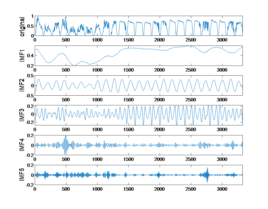
Figure 1. IMF Sub-sequences

4.3. Prediction results analysis

To further validate the accuracy and effectiveness of the proposed VMD-MSI-GWO-KELM prediction model, comparative experiments were conducted with: Single prediction model: KELM; Hybrid prediction models: VMD-KELM and VMD-newGWO-KELM. For the non-optimized KELM model, the kernel parameter \( g \) and regularization coefficient \( C \) were set to 1000 and 100, respectively. The GWO, MSI-GWO, and BWO algorithms were configured with a population size \( N \) of 20 and a maximum of 100 iterations \( {T_{max}} \) .To enhance prediction efficiency and minimize interference from different feature magnitudes, all historical sample data were normalized to ensure consistent input features. The model was trained using PV power output and the five most relevant meteorological factors, predicting PV power under three different weather conditions: sunny, cloudy, and rainy (Figure 2-4). The output was the time-series PV power generation for the target test day.

The RMSE, MAE, XMAPE, and \( {R^{2}} \) evaluation metrics for different models under different weather conditions are presented in Table 2, while Figure 3 illustrates the fitting curve for cloudy weather. All four prediction models effectively forecast PV power generation. However, the hybrid models outperform the single prediction model (KELM), demonstrating the advantages of VMD-based feature extraction and optimization algorithms. Among the hybrid models, the proposed VMD-MSI-GWO-KELM model achieves the highest prediction accuracy, further improving forecasting precision compared to other models.

Table 2. Evaluation Metrics for Various Prediction Models

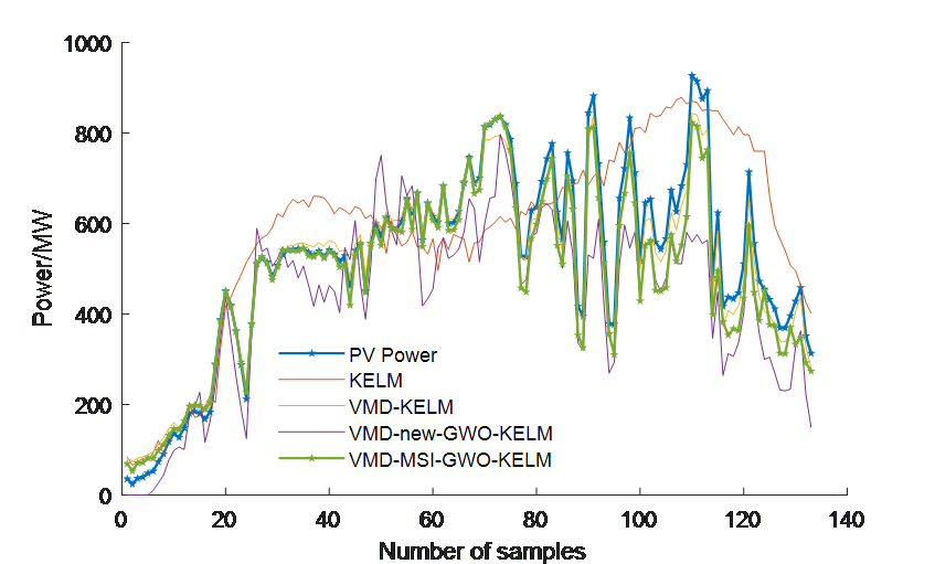
Figure 2. Comparison of Models for Sunny Weather

Figure 3. Comparison of Models for Rainy Weather

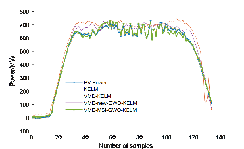
Figure 4. Comparison of Models for Cloudy Weather

5. Conclusion

This paper proposes a combined photovoltaic power prediction model, GMM-MSI-GWO-KELM, and verifies the effectiveness of this method through actual measured data.

1)The factors affecting photovoltaic power generation are selected, and similar days are chosen based on the GMM clustering results, further improving the similarity between the similar days and the forecast day.

2)A photovoltaic power prediction model based on VMD-MSI-GWO-KELM is constructed, and the parameters of KELM are optimized using a multi-strategy improved Grey Wolf Optimizer (MSI-GWO), improving both the iteration speed and prediction accuracy.

The effectiveness and accuracy of the proposed combined prediction model are verified through case studies. This prediction system demonstrates excellent performance under various weather conditions, providing a reliable technical guarantee for the accurate prediction of photovoltaic power generation and the smooth operation and scheduling optimization of grid-connected systems.

References

[1]. Ai, L., Si, J. L., & Chen, X. J. (2024). Current development status and prospects of China’s photovoltaic power generation industry [J/OL]. Hydropower Generation, 1-6 [2025-03-20]. http://kns.cnki.net/kcms/detail/11.1845.TV.20250319.1742.006.html
[2]. Wang, S. B., Wang, K., & Sun, S. M. (2025). Analysis and review of ultra-short-term photovoltaic power forecasting technology [J]. Shandong Electric Power Technology, 52(02), 55-64. DOI:10.20097/j.cnki.issn1007-9904.2025.02.006
[3]. Wang, R., Zhang, L. T., & Lu, J. (2024). Short-term photovoltaic power forecasting based on novel similar-day selection and VMD-NGO-BiGRU [J]. Journal of Hunan University (Natural Sciences), 51(02), 68-80. DOI:10.16339/j.cnki.hdxbzkb.2024227
[4]. Feng, J. M., Xi, W. A., & Lin, H. (2025). Short-term photovoltaic power forecasting based on clustering SABO-VMD and combined neural network [J]. Acta Energiae Solaris Sinica, 46(02), 357-366. DOI:10.19912/j.0254-0096.tynxb.2023-1681
[5]. Yao, Q. C., Xiang, W. G., & Chen, S. Y. (2025). Photovoltaic power forecasting based on ICEEMDAN-KPCA-ICPA-LSTM [J]. Journal of Power Engineering, 45(03), 374-382. DOI:10.19805/j.cnki.jcspe.2025.230777
[6]. Meng, Y. K., Xu, Y., & Wang, X. P. (2024). Study on combined forecasting model of photovoltaic output based on similar-day selection and PCA-LSTM [J]. Acta Energiae Solaris Sinica, 45(07), 453-461. DOI:10.19912/j.0254-0096.tynxb.2023-0498
[7]. Fang, C. X., Zheng, J. Y., & Zhang, Z. H. (2025). Distributed photovoltaic power forecasting method based on similar-day selection and VMD-DBO-KELM [J/OL]. High Voltage Technology, 1-11 [2025-03-20]. https://doi.org/10.13336/j.1003-6520.hve.20240792
[8]. Liu, Q. B., & Li, J. (2024). Short-term photovoltaic power forecasting based on SOM-FCM and KELM combination method (English) [J]. Journal of Measurement Science and Instrumentation, 15(02), 204-215
[9]. Shang, L. Q., Li, H. B., Hou, & Y. D. (2022). Short-term photovoltaic power forecasting based on VMD-ISSA-KELM [J]. Power System Protection and Control, 50(21), 138-148. DOI:10.19783/j.cnki.pspc.220140
[10]. Long, J., Zuo, S. L., & Xu, L. (2024). Dam deformation prediction model based on influencing factor selection and GWO-KELM [J]. China Rural Water and Hydropower, (08), 194-199+207
[11]. Chen, M., Chen, Y., & Niu, X. L. (2022). Multi-strategy improved grey wolf algorithm for solving global optimization problems [J]. Foreign Electronic Measurement Technology, 41(11), 22-29. DOI:10.19652/j.cnki.femt.2204260
[12]. Zhai, M. Q. (2022). Two-stage structural damage identification method based on improved grey wolf algorithm and artificial neural network [D]. Xiamen University. DOI:10.27424/d.cnki.gxmdu.2022.001599
[13]. Yang, C., Niu, F. J., & Han, M. L. (2025). Research on photovoltaic array fault diagnosis method based on improved grey wolf algorithm optimized extreme learning machine [J]. Power Generation Technology, 46(01), 72-82
Cite this article
Li,X. (2025). Short-term photovoltaic power generation prediction based on VMD-MSI-GWO-KELM. Advances in Engineering Innovation,16(3),75-82.
Data availability
The datasets used and/or analyzed during the current study will be available from the authors upon reasonable request.
Disclaimer/Publisher's Note
The statements, opinions and data contained in all publications are solely those of the individual author(s) and contributor(s) and not of EWA Publishing and/or the editor(s). EWA Publishing and/or the editor(s) disclaim responsibility for any injury to people or property resulting from any ideas, methods, instructions or products referred to in the content.
About volume
Journal:Advances in Engineering Innovation
© 2024 by the author(s). Licensee EWA Publishing, Oxford, UK. This article is an open access article distributed under the terms and
conditions of the Creative Commons Attribution (CC BY) license. Authors who
publish this series agree to the following terms:
1. Authors retain copyright and grant the series right of first publication with the work simultaneously licensed under a Creative Commons
Attribution License that allows others to share the work with an acknowledgment of the work's authorship and initial publication in this
series.
2. Authors are able to enter into separate, additional contractual arrangements for the non-exclusive distribution of the series's published
version of the work (e.g., post it to an institutional repository or publish it in a book), with an acknowledgment of its initial
publication in this series.
3. Authors are permitted and encouraged to post their work online (e.g., in institutional repositories or on their website) prior to and
during the submission process, as it can lead to productive exchanges, as well as earlier and greater citation of published work (See
Open access policy for details).