1. Introduction

Satellite attitude control plays a critical role in space missions, including Earth observation, interstellar exploration, space telescopes, and communication systems [1-2]. The attitude of a satellite refers to its direction relative to an inertial reference frame in three-dimensional space. This frame determines the direction of sensors, antennas, and propulsion systems; therefore, satellite attitude control requires extremely high precision. The attitude of a satellite will change over time due to internal torque control and external interference, and these changes all follow the control rotation dynamics equation.

Rotational dynamics are nonlinear, typically represented by quaternions or rotation matrices, and governed by nonlinear rigid body equations of motion. To avoid singularities or discontinuities, satellite attitudes are usually parameterised using quaternions or Euler angles, which are mathematical tools for describing 3D directions [3-4]. Rotation control is typically achieved through actuators such as reaction wheels, control torque gyroscopes, and thrusters, though these are subject to physical limitations such as torque saturation, rate constraints, and actuation delay [5-6]. In addition, accurate simulation is further complicated by external influences such as gravity gradient, drag, and solar pressure, which increase the complexity of control design [7-8].

Simplified linear time invariant (LTI) models are widely used in practice because of their mathematical tractability and suitability for controller design. These models are particularly effective for small-angle manoeuvres, where system dynamics can be reliably approximated by linearisation. Controllers such as proportional-derivative (PD) and linear quadratic regulator (LQR) have been widely adopted and have become standard in aerospace applications [9]. However, LTI-based methods neglect nonlinearities, coupling effects, and the true geometric shape of rotational motion present in large-angle rotations. These factors are particularly important for agile spacecraft, flexible-body satellites, or tasks operating at low actuation margins. In these cases, linear assumptions break down and controller performance suffers.

To overcome these limitations, recent studies have explored data-driven approaches such as neural networks (NNs), recurrent neural networks (RNNs), and Gaussian processes (GPs) trained on simulated or in-orbit telemetry data [10-11]. While these methods can achieve high predictive accuracy, their black-box nature makes physical interpretability, stability analysis, and integration with optimisation-based control frameworks (e.g., Model Predictive Control - MPC) difficult [12]. In contrast, Koopman operator theory offers a powerful alternative by enabling the modelling of nonlinear dynamical systems as linear systems in a lifted state-space [13-14]. The key idea is to transform the original system states into a higher-dimensional space of observables, where system evolution can be approximated by a linear operator (the Koopman operator), facilitating both analysis and control [15].

In this paper, we adopt a classical Koopman-based modelling approach. The lift function is constructed based on relevant domain knowledge, including quaternions, angular velocity, and their nonlinear interactions. This avoids training encoders or neural networks while still enabling global linear modelling in higher-dimensional spaces [16]. Quaternions and angular velocities are elevated to a higher-dimensional observable space composed of physically important features such as rotation matrices, interaction terms, and triangular expressions.

2. Problem formulation and data generation

This study aims to learn a predictive model of satellite attitude dynamics from purely simulated data without requiring prior knowledge of physical parameters. The satellite is modelled as a rigid body in three-dimensional space undergoing free rotation under external torques. Its rotational state is represented by a quaternion q(t) = [q₀, q₁, q₂, q₃]^T ∊ ℝ⁴ and an angular velocity vector ω(t) = [ω_x, ω_y, ω_z]^T ∊ ℝ³, forming the state vector x(t) = [q(t)^T, ω(t)^T]^T ∊ ℝ⁷.

Quaternions are preferred over Euler angles because they provide numerical stability, compactness, and freedom from singularities. Euler angles suffer from singularities such as gimbal lock, particularly when the pitch angle approaches ±90°, causing a loss of one rotational degree of freedom. In contrast, quaternions provide a globally non-singular representation of 3D rotations, ensuring smooth and continuous attitude tracking. Geometrically, a quaternion defines a rotation about an axis u ∊ ℝ³ by an angle σ via q = [cos(σ/2), u^T sin(σ/2)]^T (Figure 1), ensuring a one-to-one mapping to a rotation matrix on the special orthogonal group SO(3). Thus, quaternions allow continuous, globally valid tracking of satellite orientation.

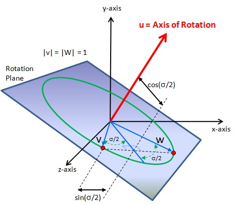
The rotation shown in Figure 1 is defined by an axis u ∊ ℝ³ and an angle σ, where the quaternion is expressed as q = [cos(σ/2), u^T sin(σ/2)]^T. Here, σ denotes the total angle of rotation about the axis u, and the diagram illustrates the relation between the rotation plane and the quaternion components. The unit vector u specifies the direction of the rotation axis in three-dimensional space, and is typically expressed in the body-fixed or inertial reference frame depending on the application.

While quaternions offer significant advantages in representing three-dimensional rotations, particularly in avoiding singularities and ensuring smooth interpolation, Euler angles remain the standard representation in many real-world satellite sensors and control systems due to their intuitive physical interpretation. In practice, raw attitude measurements are often recorded as Euler angles and then converted to quaternions for use in dynamic modelling and prediction. After prediction, the resulting quaternion outputs are transformed back into Euler angles for analysis and visualisation.

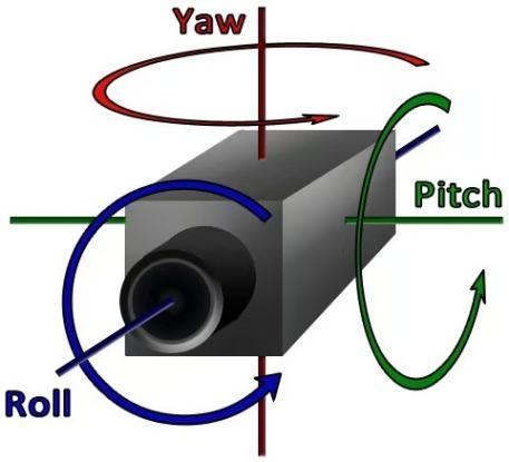
The conversion from a unit quaternion q(t) = [q₀, q₁, q₂, q₃]^T to Euler angles (ϕ, θ, ψ), corresponding to roll, pitch, and yaw, respectively, in a XYZ rotation sequence (Figure 2), is given by:

$$$ \varphi =\mathrm{a}\mathrm{r}\mathrm{c}\mathrm{t}\mathrm{a}\mathrm{n}2(2\left(q_0{q}_1+q_2{q}_3\right),1-2\left(q_2^2+q_3^2\right))$$$

$$$ \theta =\mathrm{a}\mathrm{r}\mathrm{c}\mathrm{s}\mathrm{i}\mathrm{n}2\left(2\right(q_0{q}_2-q_3{q}_1)$$$

$$$ \psi =\mathrm{a}\mathrm{r}\mathrm{c}\mathrm{t}\mathrm{a}\mathrm{n}2\left(2\right(q_0{q}_3+q_1{q}_2),1-2\left(q_2^2+q_3^2\right))$$$

The time evolution of the satellite’s rotational dynamics is governed by the rigid-body equations of motion. The quaternion dynamics follow the differential equation:

$$$ \dot{\mathit{q}}=\frac{1}{2}\mathit{Q}\left(\mathit{\omega }\right)\mathit{q}$$$

where Q(ω) ∊ ℝ^4×4 is a matrix-valued function of angular velocity given by

$Q\left(\omega \right)=\left[\begin{array}{cccc}0& -{\omega }_x& -{\omega }_y& -{\omega }_z\\ {\omega }_x& 0& {\omega }_z& -{\omega }_y\\ {\omega }_y& -{\omega }_z& 0& {\omega }_x\\ {\omega }_z& {\omega }_y& -{\omega }_x& 0\end{array}\right]$

The angular velocity evolves according to Euler’s rotational equation:

$$$ \mathit{J}\dot{\mathit{\omega }}=\mathit{J}\mathit{\omega }\times \mathit{\omega }+\mathit{\tau }$$$

where J ∊ ℝ^3×3 is the moment of inertia matrix and τ ∊ ℝ³ is the control torque input. For simulation purposes, we assume a symmetric rigid body with diagonal inertia J = 1/6 ma²I3, where m = 7.0 kg is the mass and a = 0.1 m is the edge length of the cubic satellite body. Torques are applied in all three axes, randomly generated within a maximum bound of ± τ_max = 0.001 Nm.

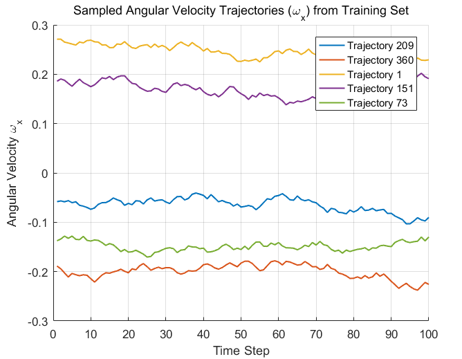
To generate training data, we simulate N = 500 random attitude trajectories using MATLAB. Each trajectory spans T = 10 s with a fixed time step Δt = 0.1 s, resulting in 100 steps per trajectory and a total of 500×100=50,000 data samples. Each simulation begins with a randomly generated initial quaternion uniformly sampled on the unit 3-sphere S³ and a randomly perturbed angular velocity vector (Figure 3). At each step, a control input τ(t) is applied, and the state is integrated forward using explicit Euler integration. After integration, the updated quaternion is re-normalised to maintain unit norm. This guarantees valid orientation representation throughout the simulation. The resulting dataset includes triples (x_t, τ_t, x_t+1) capturing the full state transition under known torque input, and is stored in structured arrays for subsequent modelling.

The simulation pipeline is fully implemented in MATLAB without external symbolic or physics solvers. The use of randomised inputs and initial conditions ensures the training data covers a wide range of dynamic behaviours, including small- and large-angle rotations, acceleration and deceleration phases, and non-trivial torque interactions. The resulting dataset provides a representative basis for learning generalisable satellite attitude dynamics in a data-driven manner.

It is important to emphasise that the goal of this data generation process is not to analytically solve or identify the governing equations of satellite attitude dynamics. Instead, the focus lies in constructing a representative dataset from a nonlinear system whose true model is assumed to be unknown. The satellite’s rotational dynamics, inherently nonlinear due to the coupling between quaternion kinematics and angular velocity evolution, cannot be directly captured using conventional linear approaches. Therefore, the Koopman operator framework is employed as a data-driven method to lift the nonlinear system into a higher-dimensional space where its evolution can be approximated linearly. In this context, data generation is essential for learning a predictive Koopman-based model, rather than for model validation or physics-informed parameter estimation.

3. Angular velocity and trajectory prediction

In this section, we introduce a method for learning a control-oriented satellite attitude dynamics model based on the Koopman operator. The Koopman framework provides a powerful way to model nonlinear systems by representing them in an enhanced observable space, where their evolution can be approximated by linear dynamics. Unlike traditional methods that require knowledge of physical laws and system parameters, the Koopman approach uses observed trajectory data to discover potential representations of nonlinear dynamic linear evolution. This feature makes it particularly suitable for integration with linear control frameworks such as MPC while maintaining high prediction fidelity.

Formally, let the original system state be denoted by x_t ∊ ℝⁿ, and control input τ_t ∊ ℝ^m_. The true system evolution is governed by a nonlinear dynamical system x_t+1 = f(x_t, τ_t). In the Koopman framework, the state is lifted via a function g(x_t+1) ∊ℝ^p, where p > n, such that the dynamics in the lifted space can be approximated by a linear system:

$$$ \text{g}\left({\text{x}}_{\text{t}\text{+1}}\right)\text{ = }\text{A}\text{g}\left({\text{x}}_{\text{t}}\right)\text{ + }\text{B}\text{τ}\text{t}$$$

where A ∊ ℝ^p×p and B ∊ ℝ^p×m are the Koopman operator matrices to be identified from data.

To construct the lifting function g(x_t), we designed a set of observable features that map the original satellite state into a higher-dimensional latent space in which the nonlinear rotational dynamics evolve approximately linearly. The original state x(t) ∊ℝ⁷ comprises a unit quaternion q(t) = [q₀, q₁, q₂, q₃]^T, representing the satellite’s orientation, and an angular velocity vector ω(t) = [ω_x, ω_y, ω_z]^T. The lifting function g(x_t) ∊ℝ⁴¹ is constructed to preserve physical interpretability while introducing sufficient nonlinear structure for accurate approximation of the dynamics using a linear Koopman operator.

The lifted state includes several categories of features. First, we retain the original state components q and ω, providing the model with a baseline representation of the orientation and rotational velocity. Second, we embed rotational geometry by converting the quaternion into a 3×3 direction cosine matrix R(q), derived from the quaternion q(t) = [q₀, q₁, q₂, q₃]^T, which is used to embed orientation into the lifted state. Each entry of R(q) represents the cosine of the angle between body-fixed and inertial axes. To incorporate it into the Koopman framework, R(q) is reshaped into a 9-dimensional vector, providing a compact and globally valid representation of orientation that captures nonlinear rotational coupling for better approximation in the lifted linear space. The direction cosine matrix is derived from the quaternion as follows:

$R\left(q\right)=\left[\begin{array}{ccc}1-2q_2^2-2q_3^2& 2q_1{q}_2-2q_0{q}_3& 2q_1{q}_3-2q_0{q}_2\\ 2q_1{q}_2-2q_0{q}_3& 1-2q_1^2-2q_3^2& 2q_2{q}_3-2q_0{q}_1\\ 2q_1{q}_3-2q_0{q}_2& 2q_2{q}_3-2q_0{q}_1& 1-2q_1^2-2q_2^2\end{array}\right]$

This allows the model to access the global rotational alignment between the body and inertial frames without suffering from singularities common to Euler angles.

To further enhance the model’s capacity to capture nonlinearities, we introduce higher-order features including the squared components of both quaternions and angular velocities: q₀², q₁², q₂², q₃² and ω_x², ω_y², ω_z². These quadratic terms allow the linear model to internally represent second-order nonlinear interactions that commonly arise in rotational dynamics, such as energy-related quantities. Additionally, to capture the nonlinear interactions between orientation and rotational velocity, we explicitly construct 12 cross-product terms between quaternion components q(t) = [q₀, q₁, q₂, q₃]^T and angular velocity components ω(t) = [ω_x, ω_y, ω_z]^T, namely: q₀ω_x, q₀ω_y, q₀ω_z, q₁ω_x, q₁ω_y, q₁ω_z, q₂ω_x, q₂ω_y, q₂ω_z, q₃ω_x, q₃ω_y, q₃ω_z. These terms are included in the lifted state to enhance the expressive capacity of the model and help the linear predictor capture rotational coupling effects more accurately.

Lastly, to capture non-polynomial and periodic nonlinearities inherent in rotational dynamics, we include trigonometric terms sin(ω_x), sin(ω_y), sin(ω_y), cos(ω_x), cos(ω_y), cos(ω_z) in the lifted state. These features enable the model to approximate periodic effects more effectively and reflect the cyclical nature of angular motion, which are otherwise poorly represented by polynomial observables.

Combined, the lifting function yields a 41-dimensional observable vector:

$g\left(x\right)=[q;\omega ;\vec{v}ec\left(R\left(q\right)\right);q^2;{\omega }^2;q\omega ;\sin \left(\omega \right);\cos \left(\omega \right)]\in {\mathbb{R}}^{41}$

This effectively embeds the state into a space rich enough to capture the essential nonlinear dynamics while preserving linear evolution under the Koopman operator. This construction enables the model to learn globally consistent, interpretable dynamics from purely data-driven observations, facilitating long-term prediction and control design without explicit knowledge of the underlying physics.

With this lifting scheme, we construct a dataset of transition tuples (x_t, τ_t, x_t+1), where each state x_t is mapped into a higher-dimensional lifted state g(x_t) ∊ ℝ^p. We define: G = [g(x₁), g(x₂), ..., g(x_N)] ∊ ℝ^p×N: the matrix of lifted current states, U = [τ₁, τ₂, ...,τ_N] ∊ ℝ^m×N: the matrix of corresponding control inputs, G’ = [g(x₁), g(x₂), ..., g(x_N+1)] ∊ ℝ^p×N: the matrix of lifted next states.

These matrices are constructed by collecting all simulation data across the trajectories, resulting in a total of N = 50000 transitions.

The Koopman matrices A ∊ ℝ^p×p and B ∊ ℝ^p×m are then learned by solving the following least-squares regression problem:

$$$ {}_{\text{A}\text{,}\text{B}}{}^{\text{min}}\text{||}\text{G}\text{’ – }\text{AG}\text{ – }\text{BU}{\text{||}}_{\text{F}}^{\text{2}}$$$

Notably, this Koopman model is trained entirely on data generated by the physics-based simulator, without relying on the explicit knowledge of the inertia matrix J or environmental disturbances. The learned Koopman model can then be used for long-term prediction of satellite attitude evolution, which we evaluate in the next section.

To evaluate the performance of the Koopman-based model in predicting satellite rotational dynamics, we conducted tests on three unseen trajectories, each consisting of 100 time steps. The results are presented in both graphical and quantitative forms. For each trajectory, we compared the predicted angular velocity ω(t) = [ω_x, ω_y, ω_z]^T and the corresponding orientation, represented in terms of Euler angles, against ground truth data.

In all three trajectories, the predicted angular velocities closely track the ground truth, as illustrated in the upper panels of Table 1. Despite some small fluctuations, the trends and magnitudes of ω_x, ω_y and ω_z are well preserved, indicating that the Koopman model successfully captures the underlying nonlinear rotational dynamics. The corresponding mean squared errors (MSEs) are extremely small, on the order of 10^-21, further confirming the precision of the model in short-horizon prediction tasks.

The lower panels of Figure 4 display the predicted versus true Euler angles for each trajectory. The agreement is visually compelling, with the predicted trajectories almost indistinguishable from the ground truth in many cases. For example, in Trajectory 1, the predicted yaw, pitch, and roll curves remain tightly aligned throughout the time horizon, with MSE values of 0.0048, 0.0012, and 0.0011 radians squared, respectively. Similar performance is observed in Trajectories 2 and 3, with slight variations depending on the complexity and rotational energy of the test motion. In Trajectory 2, which involves more significant pitch and roll changes, the MSEs are correspondingly higher (e.g., 0.0158 for Pitch), yet the predicted orientation still closely mirrors the true trajectory.

Overall, the results demonstrate that the Koopman-based modelling framework, trained on 50,000 randomly generated samples via MATLAB simulations, is capable of generalising to previously unseen rotational behaviours with high fidelity. The successful transformation from quaternion states to Euler angles not only facilitates interpretability but also highlights the model’s ability to preserve both rate and orientation accuracy across different test cases. This consistency across multiple degrees of freedom and motion profiles indicates the robustness and effectiveness of the Koopman operator framework in learning satellite attitude dynamics.

The results demonstrate extremely low prediction error for angular velocity (on the order of 10^-21), and consistently small errors for Euler angles, indicating accurate reconstruction of satellite attitude dynamics.

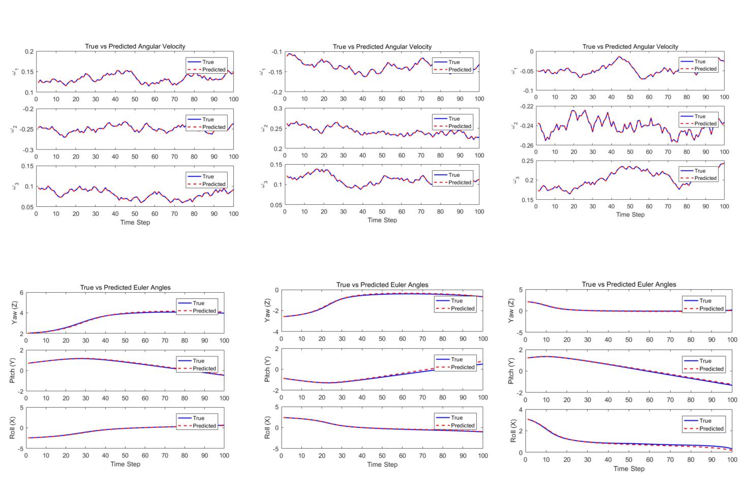
In Figure 4, the plots are arranged from left to right corresponding to Trajectory 1, Trajectory 2, and Trajectory 3. For each trajectory, the top three plots show the time evolution of angular velocity components (ω_x, ω_y, ω_z), while the bottom three plots depict the predicted Euler angles (yaw, pitch, roll). Solid blue lines represent the true values, and dashed red lines represent the predicted values.

4. MPC framework for angular velocity

This section will integrate the learned models into the MPC framework. The control objective is to asymptotically drive the angular velocity of the satellite to zero from a given initial state, thereby achieving attitude stability and angle maintenance. The controller is constructed using the previously identified Koopman linear model, characterised by the system matrices A and B, and adopts a standard quadratic cost function over a finite prediction horizon T:

$$$ {}_{{\text{u}}_{\text{0}}\text{:}\text{T}\text{-1}}{}^{\text{min}}\sum \text{k}\text{=}{\text{0}}^{\text{T}\text{-1}}\text{(}\text{||}\text{g}\text{k-}\text{g}\text{ref}{\text{||}}_{\text{Q}}^{\text{2}}\text{+||}{\mathit{\tau }}_{\text{k}}{\text{||}}_{\text{R}}^{\text{2}}\text{)}$$$

$$$ {\text{s.t. }\text{g}}_{\text{k+1}}\text{ = }\text{A}\text{g}\left({\text{x}}_{\text{t}}\right)\text{ + }\text{B}{\text{τ}}_{\text{t}}$$$

where g_k = g(x_k) denotes the lifted state at time step k, and gref is the reference lifted state corresponding to zero angular velocity in the original system space. The weighting matrices Q and R penalise state deviation and control effort, respectively. The optimisation problem is solved using MATLAB’s quadprog solver in a receding horizon manner, applying only the first optimal control input at each step and updating the state accordingly for the next iteration.

Under the proposed Koopman-MPC framework, the satellite’s angular velocity can be effectively stabilised. As shown in Figure 5, all three angular velocity components converge toward zero within a short time horizon, reflecting the controller’s ability to suppress rotational motion and maintain attitude stability. This result highlights the feasibility of embedding Koopman-based models into predictive control frameworks to achieve real-time regulation of satellite dynamics, without resorting to the full nonlinear model. It also validates the linear predictive structure obtained via Koopman lifting as a viable tool for practical control applications.

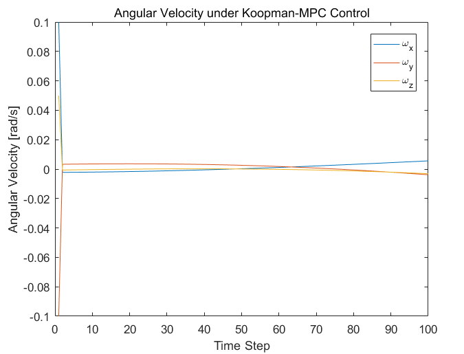
The three curves shown in Figure 5 represent the angular velocities around the x-, y-, and z-axes (ωₓ, ωᵧ, and ω_z). The results show that the controller effectively drives the angular velocity toward zero, indicating successful stabilisation.

5. Comparison of model performance

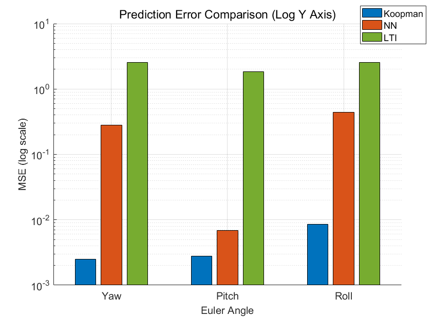
Prediction performance of different modelling approaches on spacecraft attitude dynamics was compared across three models: the Koopman operator-based model, a feedforward neural network (NN), and a linear time-invariant (LTI) system. Each model was tested on the same trajectory data to predict Euler angles (yaw, pitch, roll), and their accuracy was quantitatively assessed using the mean squared error (MSE).

As shown in Figure 6, the horizontal axis represents the three Euler angle components, while the vertical axis depicts the MSE on a logarithmic scale. It is evident that the Koopman-based model achieves the best overall performance, maintaining errors in the range of 10^-3 to 10^-2 across all directions. The prediction accuracy for the pitch angle is particularly high, suggesting relatively stable system behaviour along that axis.

The neural network model also performs well on the pitch direction (MSE ≈ 7.8 ×10^-3), but its performance degrades for yaw and roll, especially in the roll direction, where the MSE rises to approximately 0.47. This discrepancy may result from insufficient generalisation to sharp attitude changes or imbalanced data distribution across axes during training. Overall, the NN model captures some nonlinear dynamics but exhibits greater variance in performance.

In contrast, the LTI model produced significantly larger prediction errors at all Euler angles, with an MSE value of approximately 10⁰. Especially in roll prediction, it showed the lowest accuracy (MSE ≈ 2.04), indicating that the linear model structure failed to consider the inherent nonlinearity of the system. This result is consistent with the visual comparison between the predicted trajectory and the actual trajectory.

6. Conclusion

This paper proposes a data-driven modelling method for satellite attitude dynamics using the Koopman operator. By using specially designed observable functions, the original nonlinear system state composed of quaternions and angular velocities is elevated to a higher-dimensional space. This framework is suitable to some extent for scenarios where it is difficult to accurately identify the system, such as early task stages or reconfigurable satellite structures. The Koopman model learned has high prediction accuracy for angular velocity and attitude. In addition, this method provides physical interpretability by using a quaternion-based lift. These results indicate the potential of the Koopman operator as a satellite dynamics modelling tool in situations where classical models are difficult to construct or maintain.

References

[1]. Wie, B. (2008). Space vehicle dynamics and control (2nd ed.). AIAA Education Series.
[2]. Wertz, J. R. (1978). Spacecraft attitude determination and control. Springer.
[3]. Kuipers, J. B. (1999). Quaternions and rotation sequences. Princeton University Press.
[4]. Markley, F. L., & Crassidis, J. L. (2014). Fundamentals of spacecraft attitude determination and control. Springer.
[5]. Hughes, P. C. (1986). Spacecraft attitude dynamics. Dover Publications.
[6]. Schaub, H., & Junkins, J. L. (2009). Analytical mechanics of space systems (2nd ed.). AIAA.
[7]. McInnes, C. R. (1999). Solar sailing: Technology, dynamics and mission applications. Springer.
[8]. Bate, B. L., Mueller, D. D., & White, J. E. (1971). Fundamentals of astrodynamics. Dover Publications.
[9]. Psiaki, M. (2001). Attitude-determination filtering via extended Kalman filtering.Journal of Guidance, Control, and Dynamics, 24(6), 1187–1195.
[10]. Diaz, S. K., & Linares, R. (2021). Data-driven learning of satellite attitude dynamics using recurrent neural networks.Aerospace Science and Technology, 108, 106377.
[11]. Huang, H., Li, S., Wang, X., & Zhang, Y. (2022). Gaussian process regression for attitude dynamics modeling in CubeSats.Acta Astronautica, 194, 209–218.
[12]. Korda, M., & Mezić, I. (2018). Linear predictors for nonlinear dynamical systems: Koopman operator meets model predictive control.Automatica, 93, 149–160.
[13]. Bruder, D., Kaiser, E., Goldschmidt, S., Brunton, S. L., & Duraisamy, K. (2020). Data-driven identification of Koopman eigenfunctions for control.Machine Learning: Science and Technology, 2(1), 015003.
[14]. Mauroy, A., Susuki, Y., & Mezic, I. (2020). The Koopman operator in systems and control: Concepts, methodologies, and applications.Annual Review of Control, Robotics, and Autonomous Systems, 3, 67–100.
[15]. Pan, S., & Duraisamy, K. (2024). A data-driven discovery of Koopman eigenfunctions for nonlinear systems. Nonlinear Dynamics. Advance online publication.
[16]. Shi, L., & Karydis, K. (2021). Analytical construction of dictionaries for Koopman operator based representations of robotic systems.IEEE Robotics and Automation Letters, 7(2), 906–913.
Cite this article
Zhang,J. (2025). Data-driven global linear modelling of satellite attitude dynamics via Koopman operator. Advances in Engineering Innovation,16(10),1-8.
Data availability
The datasets used and/or analyzed during the current study will be available from the authors upon reasonable request.
Disclaimer/Publisher's Note
The statements, opinions and data contained in all publications are solely those of the individual author(s) and contributor(s) and not of EWA Publishing and/or the editor(s). EWA Publishing and/or the editor(s) disclaim responsibility for any injury to people or property resulting from any ideas, methods, instructions or products referred to in the content.
About volume
Journal:Advances in Engineering Innovation
© 2024 by the author(s). Licensee EWA Publishing, Oxford, UK. This article is an open access article distributed under the terms and
conditions of the Creative Commons Attribution (CC BY) license. Authors who
publish this series agree to the following terms:
1. Authors retain copyright and grant the series right of first publication with the work simultaneously licensed under a Creative Commons
Attribution License that allows others to share the work with an acknowledgment of the work's authorship and initial publication in this
series.
2. Authors are able to enter into separate, additional contractual arrangements for the non-exclusive distribution of the series's published
version of the work (e.g., post it to an institutional repository or publish it in a book), with an acknowledgment of its initial
publication in this series.
3. Authors are permitted and encouraged to post their work online (e.g., in institutional repositories or on their website) prior to and
during the submission process, as it can lead to productive exchanges, as well as earlier and greater citation of published work (See
Open access policy for details).