1. Introduction

With the trend of optimizing production capacity layout and environmental governance in the current economic and social development of China, optimizing control of industrial production has received widespread attention and research from both academia and industry [1]. In existing enterprises producing a certain electronic product, this product requires two types of components, which are paired and assembled into finished products. In the assembled finished products, if any component is defective, the finished product will definitely be defective; if both components are qualified, the assembled product may still not meet the standards. Two handling schemes are available for defective products: one is direct scrapping, and the other is disassembly, where no damage is caused to the components during disassembly, but disassembly incurs a cost.

In 2023, Yang Lei et al. proposed a data-driven model fusion method for product quality prediction in complex production processes. This method combines a holistic prediction model with a segmented prediction model, using ensemble learning techniques to address the insufficient predictive ability of individual models, thus improving prediction accuracy and enabling real-time quality monitoring. However, this method is computationally complex, requires significant computational resources, and has high demands on data quality and quantity [2]. In 2024, Mu Yaqi et al. applied the Lean Six Sigma method in optimizing the production process of R Company’s pharmaceutical products, using the DMAIC process to precisely identify and improve key variables in the production process. This method improved production efficiency, reduced costs, and enhanced product quality [3]. However, it has a high implementation difficulty, requires professional knowledge and skills, and the DMAIC process has a long cycle, with results that are difficult to achieve in the short term. In 2021, Liu Qiang’s team proposed a production process management model suitable for the automotive parts manufacturing industry at Company A, combining Lean Production with Smart Manufacturing theories [4]. This model optimized management processes, equipment, and technology, enhancing automation levels and production efficiency. However, it involves high initial investment and strong technological dependence, requiring ongoing technical support and maintenance. Tan Bo et al. applied the PDCA cycle management model at F Garment Company, combining the 5W1H and 5M1E analysis methods to conduct in-depth analysis of quality issues in production, thereby reducing defect rates and improving customer satisfaction [5]. Despite achieving results, the PDCA cycle relies on employee execution, and each cycle takes a long time, with significant effects difficult to observe in the short term. In 2011, Gausemeier et al. proposed a universal program model for the integrated development of electromechanical products, emphasizing the collaborative cooperation between product design and production systems, improving product performance and production efficiency [6]. This method requires interdisciplinary knowledge and coordination, making implementation more complex. Tolio et al. explored the co-evolution of products, processes, and production systems, emphasizing the impact of manufacturing technology limitations on new product development and production system design, thereby improving production efficiency and product quality [7]. This process requires high technical levels and has a long implementation cycle.

This paper proposes a multi-stage decision model to address the detection and disassembly issues of components, semi-finished products, and finished products encountered by enterprises during the production of electronic products. By establishing small-sample and large-sample sampling schemes and a variable decision model for global cost minimization, the key decisions in the production process are optimized. The research results show that rational decision-making can effectively reduce production costs and improve product quality. Specific methods include probability and accumulation models, normal distribution approximation, and traversal algorithms, providing a scientific basis for actual production.

2. Sampling testing scheme

2.1. Small sample sampling testing

Since in the sampling process, the components can only be classified into two categories: qualified and defective, the sampling process follows a binomial distribution pattern [8]. For a given sample size \( n \) and defect probability \( p \) , the probability of selecting defective components \( k \) from \( n \) samples is expressed as:

To calculate the probability when the defect rate of the components exceeds the nominal value, it is necessary to establish a cumulative probability model. The probability that the defect rate exceeds the nominal value can be expressed as:

The relationship between cumulative probability and sample size is shown in Figure 1:

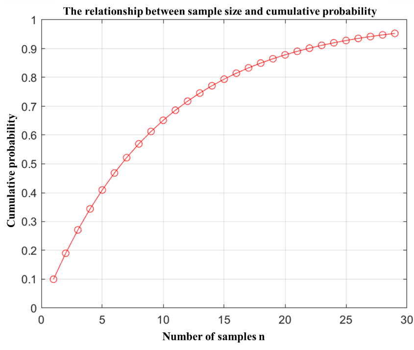
Figure 1. The Relationship Between Sample Size and Cumulative Probability

The sample size \( n \) is iteratively calculated starting from 1, gradually increasing the sample size \( n \) , and the cumulative probability corresponding to each sample size is computed. The iteration stops when the cumulative probability reaches the specified 95% confidence level, and the final sample size is determined to be 29.

From the above conclusion, it can be seen that when the sample size is 29, the defect rate of the components can be considered to exceed the nominal value with 95% confidence, leading to the rejection of the batch of components. Similarly, it is calculated that when the sample size is 22, the defect rate of the components does not exceed the nominal value with 90% confidence, so the batch of components can be accepted.

2.2. Small sample sampling testing

According to the binomial distribution pattern \( X~B(n,{p_{0}}) \) \( X~B(n,{p_{0}}) \) , the mean of \( X \) is \( n{p_{0}} \) , and the variance is \( \sqrt[]{n{p_{0}}(1-{p_{0}})} \) .

When the sample size is sufficiently large, based on the Central Limit Theorem, the components in the sampling process can be approximated as following a normal distribution pattern [9]. It is then converted into a standard form as follows:

By transforming it, we obtain:

The relationship between \( n \) and \( n \) \( {p_{1}} \) is shown in Figure 2:

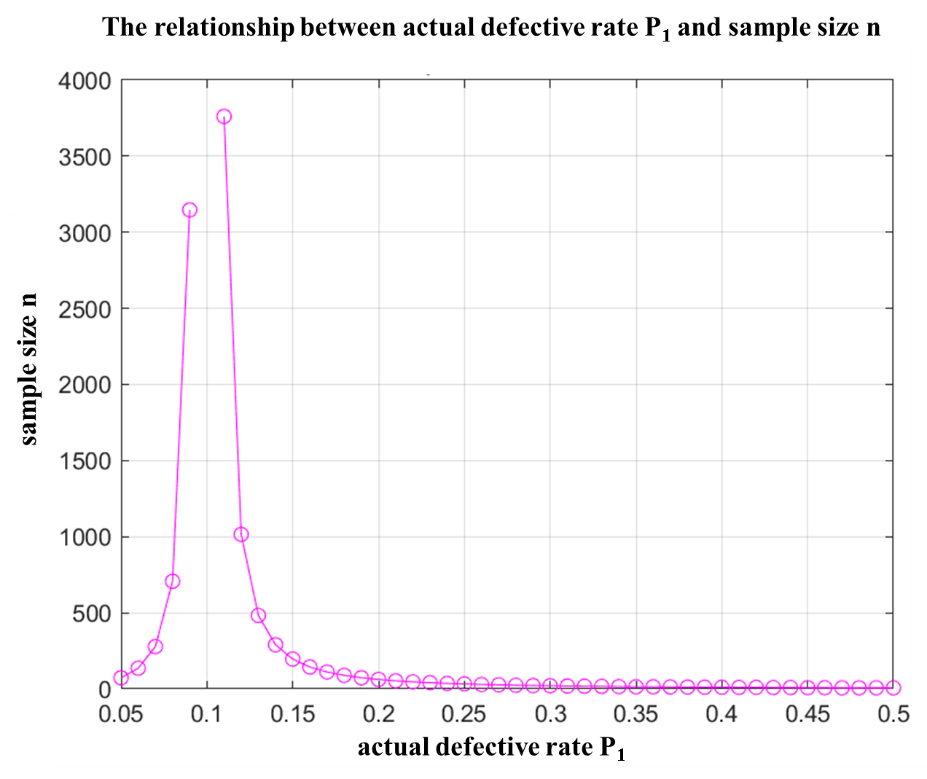
Figure 2. Relationship Between Actual Defect Rate \( {p_{1}} \) and Sample Size \( n \)

Define the error tolerance as:

Since the general error range is \( 1\%~5\% \) \( 1\%~5\% \) , the step size \( ε \) is set to 0.01. Then, using a traversal algorithm, the sample size \( ε \) corresponding to the error tolerance is obtained when the defect rate is \( 1\%~5\% \) \( 1\%~5\% \) . The final results obtained through programming are shown in the table below:

Table 1. Sample Sizes Corresponding to Different Error Tolerances

3. Cost minimization decision model

In the production process of an enterprise, decisions are made at various stages, with the goal of reducing the enterprise’s costs through reasonable decision-making. Therefore, the final cost can be considered as the basis for the final decision-making process, meaning that the ultimate decision should minimize the final cost [10,11].

Considering that there are four decision-making stages, which are as follows: whether to test Part 1, whether to test Part 2, whether each assembled finished product should be tested, and whether to disassemble defective finished products detected during testing. Use a \( 0-1 \) \( 0-1 \) decision variable \( {k_{i}} \) to determine whether each decision should be implemented:

\( {k_{1}}=\begin{cases}1,if Part 1 is tested \\ 0,if Part 1 is not tested\end{cases} \) \( {k_{2}}=\begin{cases}1,if Part 2 is not tested \\ 0,if Part 2 is not tested\end{cases} \) \( {k_{3}}=\begin{cases}1,if the assembled finished product is tested \\ 0,if the assembled finished product is not tested\end{cases} \) \( {k_{4}}=\begin{cases}1,if defective finished products detected are disassembled \\ 0,if defective finished products detected are not disassembled\end{cases} \)

Since different decisions at each stage lead to changes in the cost calculation method, each decision basis and the associated costs are analyzed separately.

3.1. Decision design for each stage

In the first stage, the testing cost for parts \( {C_{1}} \) is denoted as \( {C_{1}}={k_{1}}∙{x_{3}}+{k_{2}}∙{x_{6}} \) \( {C_{1}}={k_{1}}∙{x_{3}}+{k_{2}}∙{x_{6}} \) , where \( {x_{3}} \) \( {x_{3}} \) and \( {x_{6}} \) \( {x_{6}} \) represent the costs for testing Part 1 and Part 2, respectively.

After testing the parts, the number of finished products is given by:

Where \( {x_{1}} \) \( {x_{1}} \) denotes the defect rate of Part 1 and \( {x_{2}} \) denotes the defect rate of Part 2.

Therefore, the assembly cost for the finished products \( {C_{2}} \) should be: \( {C_{2}}=P∙{x_{8}} \) \( {C_{2}}=p∙{x_{8}} \) , where \( {x_{8}} \) is the assembly cost per finished product.

The cumulative cost for the first stage is:

After the parts are assembled, they enter the second stage. In the second stage, we first need to consider whether the assembled finished products should be tested. The testing cost generated is \( {C_{3}} \) \( {C_{3}} \) .

Where \( {x_{9}} \) \( {x_{9}} \) is the cost of testing the assembled finished products.

In the third stage, all finished products are defective, including the defective products detected in the second stage and the defective products returned by the user in the fourth stage. For the disassembly process, if disassembly occurs, the two parts might be reused. If disassembly does not take place, the two parts need to be repurchased. This corresponds to a risk of loss, i.e., an increase or decrease in cost.

Let \( kk=min{\lbrace 1-{x_{1}},1-{x_{4}}\rbrace } \) \( kk=min{\lbrace }1-{x_{1}},1-{x_{4}}\rbrace \) , and if both parts are of good quality, reassembling them may result in a qualified finished product. Therefore, the loss risk is: \( ({x_{2}}+{x_{5}})∙kk∙(1-{x_{7}}) \) .

If disassembly does not take place, there will be no cost in this stage. If disassembly occurs, a disassembly fee \( {C_{4}} \) \( {C_{4}} \) is generated:

Where \( {x_{12}} \) is the disassembly fee and \( J \) is the defect rate of the actual finished product.

The cumulative cost for the third stage is:

In the fourth stage, there is only one scenario: if no testing was conducted in the second stage, the assembled finished products directly enter the market. In this case, the user may receive defective products, and since the company will unconditionally exchange them, a loss \( {S_{6}} \) \( {S_{4}} \) from the exchange process will occur. This exchange loss can be represented as:

Where \( 1-{k_{3}} \) \( 1-{k_{3}} \) indicates that if no testing was performed in the second stage, no exchange loss occurs. Otherwise, exchange loss is incurred.

Based on the comprehensive analysis of each stage, the decision-making model for the final cost \( S \) \( S \) , using \( 0-1 \) \( 0-1 \) decision variables, is:

3.2. Exhaustive search algorithm

The Exhaustive Search Algorithm is a method that finds the optimal solution by enumerating all possible solutions [12,13]. It is suitable for problems with a small scale and limited solution space. The basic idea of the Exhaustive Search Algorithm is to systematically examine each possible solution and select the optimal one that satisfies specific conditions.

The global minimum cost \( S \) for the entire stage is derived using the Exhaustive Search Algorithm, from which the decision schemes that minimize the cost under different conditions are obtained. The specific decision schemes and related indicator results are shown in Table 2.

Table 2. Comparison Table of Cost Optimization Schemes Under the Multi-Stage Decision Model

Note: 0 means no detection/no disassembly; 1 indicates that inspection/dismantling is performed.

This result shows that, in the parts detection phase, the decision criterion is to compare the detection cost with the assembly cost of defective products. Taking part 1 as an example, the cost of not performing the detection is lower. Although this may affect subsequent results, the assembly cost of defective products is less than the detection cost, so choosing not to detect is reasonable. Similarly, the situation for part 2 supports this decision. In the finished product inspection phase, the decision is made by comparing the inspection cost with the replacement loss. For situations with a high defect rate, the cost of not inspecting is lower than the inspection cost, so not inspecting is appropriate. The analysis also shows that the decision of whether to disassemble the defective products can be determined by comparing the disassembly cost with the risk of loss. Overall, the decisions regarding the inspection of parts and finished products should be based on a cost-benefit analysis to achieve the optimal result.

4. Cost minimization decision model

When there are multiple production processes \( m \) and different assembly scenarios \( n \) for parts, as shown in Figure 3:

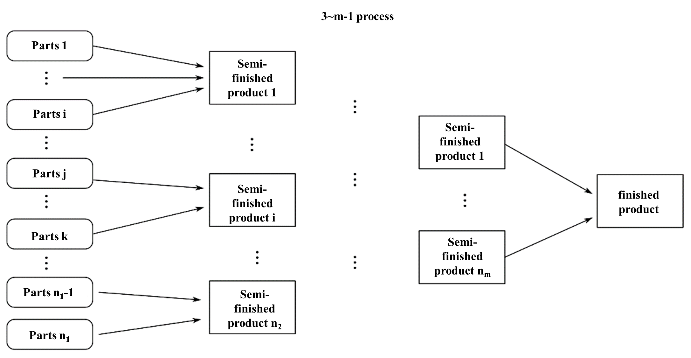
Figure 3. Multiple Production Processes \( m \) and Various Part Assembly Scenarios \( n \)

In actual production, every product must undergo multiple processes and require various parts, with each process having certain interdependencies. When considering multi-process and multi-part decision-making problems, the computation becomes extremely large, making it difficult to calculate the global minimum cost. Therefore, the model is simplified by representing the global minimum cost as the sum of the stage minimum costs from each phase.

4.1. Cost analysis

In production, the cost of purchasing parts is essential, and there is an initial required purchase cost for each part, denoted as:

Where \( {B_{j}} \) \( {B_{j}} \) represents the purchase unit price of the \( j \) \( j \) -th part.

For inspection costs, they can be compared with the cost of assembling defective products. Let the inspection cost be \( {C_{ij}} \) \( {C_{ij}} \) , the defect rate be \( {A_{ij}} \) \( {A_{ij}} \) , and the assembly cost be \( {E_{i+1j}} \) \( {E_{i+1j}} \) . If the inspection cost exceeds the cost of assembling defective products, i.e., \( {C_{ij}} \gt {A_{ij}}∙{E_{i+1j}} \) \( {C_{ij}} \gt {A_{ij}}∙{E_{i+1j}} \) , then no inspection is conducted. If the inspection cost is lower than the cost of assembling defective products, i.e., \( {C_{ij}} \lt {A_{ij}}∙{E_{i+1j}} \) \( {C_{ij}} \lt {A_{ij}}∙{E_{i+1j}} \) , then the part is inspected. The same logic applies to semi-finished products.

Thus, the inspection cost can be calculated as: \( \sum _{i=1}^{m}\sum _{j=1}^{{n_{i}}}{{C_{i}}_{j}}{{x_{i}}_{j}} \) , and the assembly cost as: \( \sum _{i=1}^{m}\sum _{j=1}^{{n_{i}}}(∏_{z=1}^{i}{k_{z}}){E_{i+1j}} \) .

For finished product inspection costs, these can be compared with the replacement loss of defective products. If the inspection cost exceeds the replacement loss for defective products, then no inspection is conducted. If the inspection cost is lower than the replacement loss, then inspection is performed.

For the defect rate of the cost \( J \) \( J \) , it can be expressed as:

If \( {C_{m+1,{n_{m+1}}}} \gt W∙J \) \( {C_{m+1,{n_{m+1}}}} \gt W∙J \) , no inspection is performed; if \( {C_{m+1,{n_{m+1}}}} \lt W∙J \) \( {C_{m+1,{n_{m+1}}}} \lt W∙J \) , inspection is performed.

The disassembly cost for defective products is given by: \( \sum _{i=2}^{m+1}\sum _{j=1}^{{n_{i}}}(∏_{z=1}^{i}{k_{z}})∙{H_{ij}}∙{y_{ij}} \) .

Using the cost minimization decision model, the replacement loss is calculated as: \( {F_{4}}=(1-{k_{3}})∙J∙\prod _{z=1}^{m}{k_{i}}∙W \) \( {F_{4}}=(1-{k_{3}})∙J∙∏_{z=1}^{m}{k_{i}}∙W \) .

4.2. Multi-stage decision model

Based on the previously discussed model with multiple production processes \( m \) and parts \( n \) , the model for two production processes and eight parts is as follows:

Where

Through calculation, the decision basis for the minimum cost is determined to be \( F=138 \) yuan.

The decision scheme is shown in Table 3:

Table 3. Decision Scheme for Multi-Part and Multi-Process Inspection and Disassembly

Note: 0 means no testing/disassembly; 1 indicates test/disassemble

5. Conclusion

This paper addresses the challenges faced by enterprises in the inspection and disassembly of parts, semi-finished products, and finished products during the production of electronic goods. A solution based on multi-stage decision analysis is proposed. The solution optimizes key decision points in the production process by designing sampling inspection strategies for both small and large samples and by constructing a decision model aimed at minimizing global costs. Various statistical and mathematical tools, including probability models, cumulative distribution functions, normal distribution approximations, and exhaustive search algorithms, are employed to calculate the lowest unit cost under different scenarios and to propose corresponding optimal decision recommendations. Experimental calculations of the relevant data demonstrate that effective decision-making can significantly reduce costs and improve product quality. Additionally, this paper explores complex decision-making problems involving multiple processing steps and various parts. By breaking down large problems into smaller ones, the process is simplified, and the sum of the minimum costs of each stage is taken as the optimal solution for overall costs. After analyzing a specific case with two production processes and eight parts, the minimum unit cost obtained is 138. The recommended decision path is to not inspect the parts and semi-finished products, but to only inspect the finished products and to implement disassembly for the semi-finished and finished products.

This study provides solid theoretical support for practical operations within enterprises. Future research should focus more on the uncertainty and risk control in the production environment to achieve deeper optimization objectives. For instance, dynamic adjustment strategies could be explored to update the decision model in real-time according to changes in the production line. Additionally, integrating big data analytics and artificial intelligence technologies could further enhance the precision and efficiency of decision-making.

References

[1]. Liu, C. (2020). Decision-making method for optimizing operation indicators in process industries based on reinforcement learning (Unpublished doctoral dissertation).
[2]. Yang, L. (2023). Data-driven model fusion for product quality prediction in complex production processes (Doctoral dissertation, Wuhan University of Science and Technology). https://doi.org/10.27380/d.cnki.gwkju.2023.000357
[3]. Mu, Y. (2024). Research on product production process optimization of R Company based on Lean Six Sigma (Doctoral dissertation, Yanshan University).
[4]. Liu, Q. (2024). Research on product production process management optimization at A Company (Doctoral dissertation, Inner Mongolia University of Finance and Economics). https://doi.org/10.27797/d.cnki.gnmgc.2024.000408
[5]. Tan, B., Zhan, H., Wu, H., et al. (2021). Analysis and improvement of production process quality factors of a garment enterprise based on PDCA. Henan University of Engineering Journal (Natural Science Edition), 33(03), 10-15. https://doi.org/10.16203/j.cnki.41-1397/n.2021.03.003
[6]. Gausemeier, J., Dumitrescu, R., Kahl, S., et al. (2011). Integrative development of product and production system for mechatronic products. Robotics and Computer Integrated Manufacturing, 27(4), 772-778.
[7]. Tolio, T., Ceglarek, D., ElMaraghy, H., et al. (2010). SPECIES—Co-evolution of products, processes and production systems. CIRP Annals - Manufacturing Technology, 59(2), 672-693.
[8]. Liu, J., & Luo, Y. (2019). Study on the field testing and sampling method for steel structures. Advances in Steel Structures, 21(05), 33-39. https://doi.org/10.13969/j.cnki.cn31-1893.2019.05.005
[9]. Hughes, P. T., Baird, H. A., Dinsdale, A. E., et al. (2002). Detecting regional variation using meta-analysis and large-scale sampling: Latitudinal patterns in recruitment. Ecology, 83(2), 436-451.
[10]. Cui, J., & Kong, Y. (2016). Research on a comprehensive decision-making model for minimizing social costs in carbon emission rights allocation between industrial sectors. China Management Science, 24(S1), 890-895.
[11]. Swaathi, K., Vang, M. J., Bach, M. J., et al. (2022). A cost-minimisation analysis of performing point-of-care ultrasonography on patients with vaginal bleeding in early pregnancy in general practice: A decision analytical model. BMC Health Services Research, 22(1), 55.
[12]. Ren, Y. (2021). Research on product production process optimization of HF company GPT products based on Lean production (Doctoral dissertation, Xi’an University of Architecture and Technology). https://doi.org/10.27393/d.cnki.gxazu.2021.001256
[13]. Li, M. (2021). Smart cloud logistics control and management using a node group traversal simulation algorithm. Journal of Guiyang University (Natural Science Edition), 16(02), 6-10. https://doi.org/10.16856/j.cnki.52-1142/n.2021.02.002
[14]. Zhang, S. (Ed.). (2018). Probability theory and mathematical statistics. Science Press.
[15]. Hu, L., & Sun, X. (Eds.). (2020). MATLAB mathematical experiments (3rd ed.). Higher Education Press.
[16]. Jiang, Q., Xie, J., & Ye, J. (2018). Mathematical models (5th ed.). Higher Education Press.
Cite this article
Li,J.;Song,X. (2025). Based on multi-stage decision analysis in the production process. Advances in Operation Research and Production Management,3,37-44.
Data availability
The datasets used and/or analyzed during the current study will be available from the authors upon reasonable request.
Disclaimer/Publisher's Note
The statements, opinions and data contained in all publications are solely those of the individual author(s) and contributor(s) and not of EWA Publishing and/or the editor(s). EWA Publishing and/or the editor(s) disclaim responsibility for any injury to people or property resulting from any ideas, methods, instructions or products referred to in the content.
About volume
Journal:Advances in Operation Research and Production Management
© 2024 by the author(s). Licensee EWA Publishing, Oxford, UK. This article is an open access article distributed under the terms and
conditions of the Creative Commons Attribution (CC BY) license. Authors who
publish this series agree to the following terms:
1. Authors retain copyright and grant the series right of first publication with the work simultaneously licensed under a Creative Commons
Attribution License that allows others to share the work with an acknowledgment of the work's authorship and initial publication in this
series.
2. Authors are able to enter into separate, additional contractual arrangements for the non-exclusive distribution of the series's published
version of the work (e.g., post it to an institutional repository or publish it in a book), with an acknowledgment of its initial
publication in this series.
3. Authors are permitted and encouraged to post their work online (e.g., in institutional repositories or on their website) prior to and
during the submission process, as it can lead to productive exchanges, as well as earlier and greater citation of published work (See
Open access policy for details).