1. Introduction

Quantum computing is advancing to meet the growing demand for computational efficiency in modern science and technology. Through the usage of quantum states, the field offers breakthrough applications and insights, including quantum cryptography for ultra-secure classical information transmission, quantum error correction for preserving quantum coherence amidst noise, and quantum computation for efficient processing through controlled quantum evolution [1]. Our paper mainly focuses on quantum error correction.

In recent years, the problem of noise has emerged as a predominant obstacle in the advancement of universal quantum computers. Quantum decoherence, which refers to the preservation of quantum states despite the interference of noise，is necessary in order to keep quantum computing reliable. Nowadays, experimental efforts have been made to simulate quantum computations on small-scale devices, aiming to achieve the quantum decoherence [2]. Unfortunately, these experiments are usually complicated and challenging. Though the experiments are difficult, quantum error-correcting codes offer a promising solution, which is also the reason for the exploration in our study.

Detecting effective quantum error-correcting codes involves various methodologies to compare and select optimal approaches: methods for encoding a single qubit to correct multiple errors [3]; the use of entire classes of codes makes the codes for multiple-correction of many qubits efficient [4,5]; in [6], the author provides efficient quantum error corrections codes and discusses techniques for manipulating codes and guessing new codes.

In our paper, we introduce a novel but useful method for representing qudits through polynomials. Though previous applications are limited to simpler square lattice codes, we do extend this approach to more complex scenarios in Cayley graphs, and give an example of the situation on the Cayley graph of dihedral group  $$ D_4$$ .

We outline topics of individual sections. Section 2 introduces basic concepts of quantum information. Section 3 introduces Groups and Graphs, especially Cayley graphs. Section 4 discusses the definitions and examples of stabilizer codes. Section 5 discusses the existing representation of stabilizer codes and our own innovations of stabilizer codes for a more complex group or in a more complicated graph. Section 6 shows an example of using our innovative method to find the stabilizer codes.

2. Quantum information

Quantum information systems improve the quantum computing through the usage of quantum mechanical phenomena to enhance computational efficiency. Moreover, we would like to highlight the fundamental characteristics of quantum information, which encompass quantum superposition and entanglement.

Property.1Quantum information is uncertain.

In classical computers, data are stored, sent, received, and processed in the string of form of bits, which is either 0 or 1. Contrary to that, quantum information systems demonstrate a significantly different situation. Initially, quantum bits, also known as qubits, are present in a superposition of multiple quantum states. Later, quantum collapse may be precipitated by observation in quantum information, resulting in a state change. This collapse is the collapse of the wave function, which represents to the mathematical representation of the quantum state of a certain quantum system. Specifically, collapse refers to the transformation of a wave function from a superposition of multiple quantum states to a single state as a result of observation. Quantum supervision theory points out that the quantum states of qubits is the state in a linear combination of state 0 and state 1 instead of either 0 or 1. Observing a qubit can change its superposition state to either 0 or 1. Hence, the qubit will transition from the state of superposition to a state of definitiveness. As an illustration, consider a qubit system consisting of 500 qubits. When doing the first observation, 300 of them might be 0. However, in the second observation, the value might change to 200. In essence，every observation and measurement will result in diverse outcomes.

Property.2Quantum information is not local.

According to the theory of quantum entanglement, the quantum state of each particle is not independently determined by itself, but rather can only be described in a global context. If there is a pair of entangled particles, measurement and observation will determine the quantum state of one of them. This allows us to infer the state of the other particle based on their global state. This indicates that in a quantum information system, every qubit’s quantum state is affected by the others. Consider, for example, a pair of qubits, consisting of 0 and 1. In a quantum information system with several qubits, the quantum state of one qubit influences the states of the other qubit, leading to a complex entangled system[7].

2.1. Basic concepts

2.1.1. Qubit

In classical computer, data is stored as strings of bits (0s or 1s), and always represented as vectors over  $$ Z_2$$ . In quantum computing, as used lots of times before, the basic unit of quantum information is called qubits, and the state is usually written in  $$ |\psi ⟩$$ , which uses Dirac notation. “ $$ | ⟩$$ ” and “ $$ ⟨ |$$ ” are two basic representations in Dirac notation. “ $$ | ⟩$$ ” represents a column vector and “ $$ ⟨ |$$ ” represents a row vector. In this essay, we mainly use “ $$ | ⟩$$ ” . For example, the standard basis vectors of a single qubit  $$ |0⟩$$  and  $$ |1⟩$$  can be written as  $$ |0⟩=\left[\begin{array}{c}1\\ 0\end{array}\right]$$  and  $$ |1⟩=\left[\begin{array}{c}0\\ 1\end{array}\right]$$ . Note that if there we want to represent three qubits, including  $$ |0⟩$$ ,  $$ |0⟩$$ , and  $$ |1⟩$$ , we can use  $$ |001⟩$$ . This is an example of utilizing Dirac notation to represent multiple qubits. The normalized representation of qubit state is

$$ {\left|\alpha \right|}^2+{\left|\beta \right|}^2=1,$$(1)

where  $$ {\left|\alpha \right|}^2$$  and  $$ {\left|\beta \right|}^2$$  are the probabilities of obtaining  $$ 0$$  and  $$ 1$$  respectively.  $$ \alpha $$  and  $$ \beta $$  are used in the representation of an arbitrary single-qudit state:[8]

$$ |\psi ⟩=\alpha |0⟩+\beta |1⟩=\left[\begin{array}{c}\alpha \\ \beta \end{array}\right]$$(2)

There is a basic criteria for quantum error correction about the qubits and environment. The initial state of an environment is denoted by  $$ {|0 ⟩}_E$$ . A unitary transformation is used to characterize the evolution of a qubit and its environment:

 $$ |0⟩\otimes {|0⟩}_E\to |0⟩\otimes {|00⟩}_E+|1⟩\otimes {|1⟩}_E,$$ 

 $$ |1⟩\otimes {|0⟩}_E\to |0⟩\otimes {|10⟩}_E+|1⟩\otimes {|11⟩}_E;$$ 

in which  $$ |e_{ij}⟩$$  is defined as the four states of the environment that do not need to be normalized or mutually orthogonal or mutually orthogonal[9].

2.2. Inner product space

An inner product space is a vector space denoted by  $$ \mathbf{V}$$ . The operation of  $$ \mathbf{V}$$  is inner product denoted by  $$ \left(\cdot ,\cdot \right)$$ . Here is an example. The inner product, denoted by  $$ \left(\overrightarrow{x},\overrightarrow{y}\right)$$ ,or dot product  $$ \overrightarrow{x}\cdot \overrightarrow{y}$$  of two vectors  $$ \overrightarrow{x}=\left(x_1,x_2,x_3,\dots ,x_n\right)$$  and  $$ \overrightarrow{y}=\left(y_1,y_2,y_3,\dots ,y_n\right)$$ , where  $$ \overrightarrow{x}$$  and  $$ \overrightarrow{y}$$  are two elements of Euclidean Space  $$ {\mathbb{R}}^n$$  is

$$ \left(\overrightarrow{x},\overrightarrow{y}\right)=x_1{y}_1+x_2{y}_2+x_3{y}_3+\dots +x_n{y}_n.$$(3)

There are totally 4 axioms of  $$ \mathbf{V}$$ :

Axiom.1 $$ \left(\overrightarrow{x},\overrightarrow{x}\right)\ge 0$$  when  $$ \left(\overrightarrow{x},\overrightarrow{x}\right)=0$$ ,  $$ \overrightarrow{x}=\overrightarrow{0}$$ .

Axiom.2 $$ \left(\overrightarrow{x},\overrightarrow{y}+\overrightarrow{z}\right)=\left(\overrightarrow{x},\overrightarrow{y}\right)+\left(\overrightarrow{x},\overrightarrow{z}\right)$$ 

Axiom.3 $$ \left(\overrightarrow{x},a\overrightarrow{y}\right)=a\left(\overrightarrow{x},\overrightarrow{y}\right)$$  for all  $$ a\in \mathbb{R}$$ 

Axiom.4 $$ \left(\overrightarrow{x},\overrightarrow{y}\right)=\left(\overrightarrow{y},\overrightarrow{x}\right)$$  for all  $$ \overrightarrow{x}$$ ,  $$ \overrightarrow{y}$$   $$ \in \mathbf{V}$$ .

Every inner-product space is a normed space because if there is an inner product space  $$ \mathbf{V}$$ , the map  $$ \parallel \cdot \parallel $$  defined by setting  $$ \parallel \overrightarrow{v}\parallel ={\left(\overrightarrow{v},\overrightarrow{v}\right)}^{\frac{1}{2}}$$  defines a form on  $$ \mathbf{V}$$ . When the norms are “standard norms”, the vector space is complete and in this situation, the inner-product space is called Hilbert space [10].

2.2.1. Qudit

In d-dimentional Hilbert space  $$ {\mathbb{C}}^d$$ , where  $$ d\in {\mathbb{N}}^{\mathrm{*}}$$ , where  $$ \mathbb{C}$$  is the set of complex numbers, the quantum state is called qudit.

2.3. Quantum error correction

An essential goal of quantum error correction is to minimise the harmful impact of noise on quantum information. Quantum noise refers to the elements that impact the precision of calculations performed on a quantum computer. For example, cosmic rays, radiation from mobile phones, or the magnetic field of the Earth are all the sources of quantum noise. These noises may lead to quantum error, which is the error happening in quantum algorithm, finally resulting in the error in information transferred by quantum computer. When quantum error happens, the input of a pure qudit will produce a mixed state or it will become a different pure state compared with the input one.

The codes known as Quantum Error Correcting Codes (QECC) often carry out this operation. QECC always perform 3 operations to correct the error of a quantum computing. Firstly, they encode the initial state of quantum information. Then, the diagnose errors. Finally, some recovery operations will be implemented to rectify errors.

QECC can be viewd as a mapping of  $$ k$$  qubits (a  $$ 2^k$$  dimensional Hilbert space) into  $$ n$$  qubits (a  $$ 2^n$$  dimensional Hilbert space). The encoding operation of  $$ k$$  qubits toward  $$ n$$  qubits is denoted by  $$ \left[\left[k,n\right]\right]$$ . The image of this mapping is known as the code space.

Take the situation when only one error on a single qubit at a time as an example, the first step is to encode the given logical qudit as follows:

 $$ |0⟩\to |\bar{0}⟩=\left(|000⟩+|111⟩\right)\left(|000⟩+|111⟩\right)\left(|000⟩+|111⟩\right)$$ 

 $$ |1⟩\to |\bar{1}⟩=\left(|000⟩-|111⟩\right)\left(|000⟩-|111⟩\right)\left(|000⟩-|111⟩\right)$$ 

Through the encoding process above, the data can be stored as 9 qubits.

The second process is the diagnosis of errors. Suppose the first qubit is flipped by switching  $$ |0⟩$$  and  $$ |1⟩$$ . When comparing the first and the second qubit, it is not difficult to find they are different. Note that during the process of diagnosis, the superposition state is not destroyed because the difference between the first and the second qubit is the object of measurement instead of the qubit itself. Then through comparing the first and the third qubit, we can find the first qubit disagrees with the third one. Thus, we can narrow the error to the first qudit. Finally, the recovery operation is basically flipping the first qudit. This kind of error is called a bit flip.

Another possible error in one qubit is sign flips, which is shown as follows :

 $$ |0⟩\to |\bar{0}⟩=\left(|000⟩+|111⟩\right)\left(|000⟩-|111⟩\right)\left(|000⟩+|111⟩\right)$$ 

 $$ |1⟩\to |\bar{1}⟩=\left(|000⟩-|111⟩\right)\left(|000⟩+|111⟩\right)\left(|000⟩-|111⟩\right)$$ 

Here we only need to compare whether the first sign is same as the second and the third one, thus find the error and flip the sign. A bit flip and a sign flip can be described as the operations as follows respectively:

2.4. Pauli matrix & pauli operator

The operations introduced in Section 2.3 belong to a group of matrices called Pauli matrix.

Pauli matrix includes 4 different matrices as follows [11]:

Any  $$ 2\times 2$$  matrix can be expressed as a linear combination of these four matrices. For example, if  $$ \left[\begin{array}{cc}a& b\\ c& d\end{array}\right]$$  is a  $$ 2\times 2$$  matrix, it can be expressed as follows:

where  $$ c_1$$ ,  $$ c_2$$ ,  $$ c_3$$ , $$ c_4$$  are constants determined by  $$ a,b,c,d$$  [7].

A Pauli operator is formed by taking a tensor product of Pauli matrix on a set of qudits  $$ {\mathbb{C}}^d\otimes \dots \otimes {\mathbb{C}}^d$$ . On a single qudit  $$ {\mathbb{C}}^d$$ , there are two Pauli matrices:  $$ X_d,Z_d$$  which are defined as follows:

Consider a set of orthonormal basis vectors denoted by  $$ \{|0⟩, |1⟩,\dots , |d-1⟩\}$$ . Pauli matrices  $$ X_d$$  and  $$ Z_d$$  are characterized by

$$ X_d |i⟩ =|i+1\hspace{0.33em}\hspace{0.33em}\hspace{0.33em}\mathit{mod}d⟩$$(4)

$$ Z_d|i⟩ ={\omega }^i |i⟩,$$(5)

where  $$ \omega =e^{\frac{2\pi \sqrt{-1}}{d}}$$  the primitive  $$ d$$ -th root of unity. Note that when applying  $$ X_d$$  and  $$ Z_d$$  to a graph,  $$ X_d$$  means flip symmetry operation so that the overall shape of the graph does not change, and  $$ Z_d$$  means rotation operation so that the overall shape of the graph does not change.

Pauli operators form a group denoted by  $$ \mathcal{P}$$ . The definition of group and more information about Pauli group will be discussed in section 3. Note the following important commutation relation

$$ X_d{Z}_d=\omega Z_d{X}_d.$$(6)

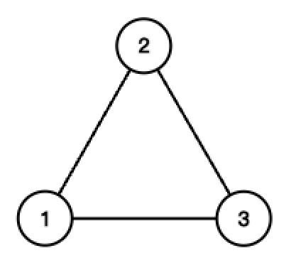
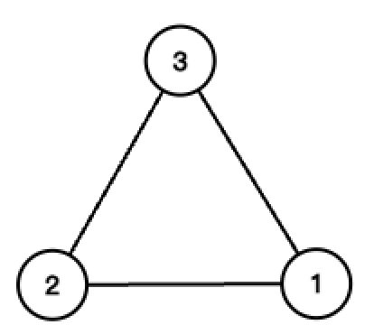
Here is an example of an equilateral triangle.

The equilateral triangle  $$ A$$  is shown in Figure 1. Specifically,  $$ Z_3 |1⟩$$  is defined as rotating  $$ \frac{2\pi }{3}$$  counterclockwise around the center point  $$ O$$  (this is also the operation of  $$ \omega $$ ), and  $$ Z_3 |2⟩$$  is defined as rotating  $$ \frac{4\pi }{3}$$  counterclockwise around the center point  $$ O$$ . Note that  $$ Z_d|n⟩$$ , where  $$ n$$  is the notation of a point of  $$ A$$ , is defined as the reflection with respect to the axis of symmetry across the center point and vertex  $$ n$$  (note that the direction of the symmetry is defined at the first time and it will not change.). For example, let the line across the center point and vertex 1 be the axis of symmetry. When there is no operations applied to the graph, this axis is denoted by  $$ X_3|1⟩$$ , which is the line perpendicular to the horizontal plane.

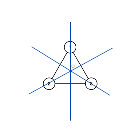
By applying the operations  $$ X_3{Z}_3|1⟩$$ , the triangle will be changed to Figure 2. However, by applying the operations  $$ Z_3{X}_3|1⟩$$ , the triangle will be changed to Figure 3. In order to transform Figure 3 to Figure 2, an extra  $$ \omega $$  operation should be applied before the operation  $$ Z_3{X}_3|1⟩$$ , that is why  $$ X_d{Z}_d=\omega Z_d{X}_d$$ .

3. Group and cayley graph

3.1. Definition of group

A group  $$ \mathbf{G}$$  is used to define a set that includes an operation, denoted by  $$ \mathrm{*}$$ , which connects two elements in the group to form the third element. This operation is called binary operation. All groups satisfy four axioms as follows:

Axiom.1 A group is closed under the operation.

After applying a binary operation, the third element formed by the two chosen elements should belong to the set which the two chosen elements belong to.

Axiom.2 Associativity is allowed in groups.

Associativity is allowed in groups. For example,  $$ \left(1+2\right)+3=1+\left(2+3\right)$$ .

Axiom.3 Identity element

The identity element  $$ e$$  satisfies that the operation of  $$ e$$  and every element in  $$ \mathbf{G}$$  will be equal to the chosen element  $$ a$$ , which is the formula:  $$ a\mathrm{*}e=e\mathrm{*}a=a$$ 

Axiom.4 Inverse element

For every element in  $$ \mathbf{G}$$ , there is an inverse element such that the operation of the chosen element  $$ a$$  and its inverse  $$ b$$  will be the identity element, which is the formula:  $$ b\mathrm{*}a=a\mathrm{*}b=e$$ .

Abelian group is also named commutative group, in which the order of two group elements does not affect the results after doing group operation, basically satisfying  $$ a\mathrm{*}b=b\mathrm{*}a$$  when  $$ a,b$$  belong to the given abelian group.  $$ \left(\mathbb{Z},+\right)$$  is an example of abelian group because  $$ a+b=b+a$$  for all  $$ a,b\in \mathbb{Z}$$ . [12]

3.2. Examples and counter-examples of group

Example.1 Set of all integers with operation  $$ +$$ :  $$ \left(\mathbb{Z},+\right)$$ 

 $$ \mathbb{Z}$$  is the set of all integers. The binary operation is addition.

Example.2 Set of Pauli operators with operation  $$ \circ $$ :  $$ \left(\mathcal{P},\circ \right)$$ 

Pauli operators over a set of qudits form a group  $$ \mathcal{P}$$ . Indeed, product of Pauli operators is still a Pauli operator. Note multiplication of Pauli operation is not necessarily commutative due to (6).

Counter-Example.1 Set of all integers with operation  $$ \times $$ :  $$ \left(\mathbb{Z},\times \right)$$ 

 $$ \mathbb{Z}$$  is the set of all integers. The binary operation is multiplication. However, it lacks an inverse that belongs to  $$ \mathbb{Z}$$ .

3.3. Definition of subgroups

A subgroup  $$ \mathbf{H}$$  is a subset of  $$ \mathbf{G}$$  which is a group, denoted by  $$ \mathbf{H}\le \mathbf{G}$$ .  $$ \mathbf{H}$$  and  $$ \mathbf{G}$$  are groups with the same binary operation [12].

Example.1  $$ \left(\mathbb{Z},+\right)\le \left(\mathbb{Q},+\right)\le \left(\mathbb{R},+\right)\le \left(\mathbb{C},+\right)$$ 

Example.2 If  $$ a\in \mathbb{N}$$  divides  $$ b\in \mathbb{N}$$ , then  $$ \left(b\mathbb{Z},+\right)\le \left(a\mathbb{Z},+\right)$$ .

3.4. Fundamental theorem of homomorphism

Given two groups  $$ \left(G_1,\circ \right)$$  and  $$ \left(G_2,\mathrm{*}\right)$$ , a mapping  $$ f:G_1\to G_2$$  is a group homomorphism if it satisfies

Here are some fundamental definitions of homomorphism:

Definition.1 If  $$ f$$  is surjective,  $$ f$$  is an epimorphism.

Definition.2 If  $$ f$$  is injective,  $$ f$$  is a monomorphism.

Definition.3 If  $$ f$$  is bijective, which means both surjective and injective,  $$ f$$  is an isomorphism. In this situation,  $$ G_1$$  and  $$ G_2$$  are isomorphic groups, denoted by  $$ G_1\cong G_2$$ .

Definition.4 If  $$ G_1=G_2$$ ,  $$ f$$  is an endomorphism, which means a homomorphism from a group to itself.

Definition.5 If  $$ G_1=G_2$$ ,  $$ f$$  is an automorphism and an isomorphism.

Another essential concept in terms of homomorphism is  $$ kernal$$  of  $$ f$$ , denoted by  $$ ker\left(f\right)$$ . If  $$ f:G_1\to G_2$$  is a homomorphism,

The image of  $$ f$$ , denoted by  $$ im\left(f\right)$$ , is the range of  $$ f$$  within  $$ G_2$$ , which is defined as

After introducing some basic definitions, we need to know one of the most important theorem involved in group, which is Group Isomorphism Theorem.

 $$ G_1$$  and  $$ G_2$$  satisfy the two following properties:

Property.1 If  $$ ker\left(f\right)$$  is a normal subgroup in  $$ G_1$$ , and  $$ im\left(f\right)$$  is a subgroup of  $$ G_2$$ ,

Property.2 Suppose  $$ H$$  is a normal subgroup of a group  $$ G$$ .  $$ f:G\to G/H$$ , given by  $$ f\left(g\right)=gH$$  for  $$ g\in G$$  is a homomorphism. Here  $$ ker\left(f\right)$$  is  $$ H$$  and  $$ im\left(f\right)$$  is  $$ G/H$$ .[12]

3.5. Group representation

Group representation theory examines homomorphisms mapping a group to the group of invertible linear transformations over vector spaces. To be more specific, it studies how abstract groups can be showed in the form of matrices and how their elements relates to linear transformations of vector spaces. Through the analysis of these representations, researches can get some helpful inspirations into the structure and properties of the group [13].

3.6. Group generators & generating set

If there is an element  $$ g\in G$$  such that  $$ G=⟨g⟩$$ , then  $$ G$$  is cyclic. Every element of  $$ G$$  can be expressed as an integer power of  $$ g$$ . In this instance,  $$ g$$  is defined as the generator of  $$ G$$ , and  $$ G$$  is generated by  $$ g$$ .

Here is an example,  $$ {\mathbb{Z}}_7$$  is cyclic because we can say it is generated by 3. All the elements of  $$ {\mathbb{Z}}_7$$  can be write in the following form:

A generating set refers to a group of elements that can be combined (including themselves, their inverses, and all possible combinations of them) to produce all the elements of an entire group. In simple terms, if a group  $$ G$$  can be generated by the elements in a set S through the group’s operation, then we say  $$ S$$  is a generating set of  $$ G$$  .

3.7. Definition of graph

According to the directed and undirected nature of the edges of the graph, graphs can be classified as directed graphs, undirected graphs, and mixed graphs. In directed graph, edges have directions, usually presented as an arrow.  $$ \left(x,y\right)$$  means the edge’s direction is from  $$ x$$  to  $$ y$$ . If the pair is not given an order and the edge has no direction，the graph is referred to as an undirected graph. A mixed graph consists of both directed edges and undirected edges.

3.8. Cayley graph

Cayley graph is a directed graph associated to  $$ \mathbf{A}$$ , denoted by  $$ {\mathbf{G}}_{A,S}$$ , where  $$ \mathbf{A}$$  is a group and  $$ S$$  is the generating set of  $$ \mathbf{A}$$ . The graph includes two primary parts:

• Vertices are elements in set  $$ \mathbf{A}$$ .

• Edges are elements in set  $$ \mathbf{A}\times \mathbf{S}$$ .

Constructing a Cayley graph is the way of producing an unbounded sequence of  $$ d$$ -regular graphs at all. The way to construct a Cayley Graph is very simple, starting by taking a group  $$ \mathbf{G}$$  and some subset  $$ \mathbf{H}$$  of  $$ \mathbf{G}$$ . We define the elements of  $$ \mathbf{G}$$  as the vertices of the Cayley graph, and the edges of the Cayley graph is the line drawn from  $$ x$$  to  $$ x\gamma $$  given that  $$ x\in \mathbf{G}$$  and  $$ \gamma \in \mathbf{H}$$ .[8]

In a Cayley graph, each edge is associated with a pair  $$ \left(a,s\right)$$ , where  $$ a\in \mathbf{A}$$  and  $$ s\in \mathbf{S}$$ . Define  $$ \iota \left(e\right)$$  as the initial vertices of the edge  $$ e$$  and  $$ \tau \left(e\right)$$  as the terminal vertex of the edge  $$ e$$ . The mapping  $$ \iota $$  and  $$ \tau $$  are specified by

Therefore, through the generator  $$ s$$ , the edge associated with the pair  $$ \left(a,s\right)$$  can run from  $$ a$$  to  $$ as$$ .

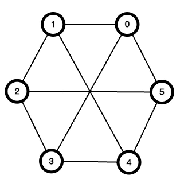
Here is an example of a Cayley graph in the sequence  $$ \left(Cay\left({\mathbb{Z}}_{2n},1,n,2n-1\right)\right)$$ . When  $$ n=3$$ , the Cayley graph  $$ \left(Cay\left({\mathbb{Z}}_6,1,3,5\right)\right)$$  is shown in Figure 4 [8]:

4. Stabilizer codes

In quantum information and theoretical condensed matter physics, stabilizer codes are often mentioned(defined below). They originate from quantum error correction, but are widely studied now as toy models for exotic quantum phases. The famous toric code model for anyons as well as the X-cube model for fractons both fall under this category.

4.1. Definition

Stabilizer codes refer to a collection of quantum codes utilized for performing quantum error correction. Given a set of qudits  $$ {\mathbb{C}}^d\otimes \dots \otimes {\mathbb{C}}^d$$ , its code space is defined as the subspace of vectors invariant under a set  $$ \mathbf{S}$$  of Pauli operators known as stabilizers. A Pauli operators on  $$ N$$  qubits can be expressed as  $$ c{O}_1{O}_2\dots O_N$$  where  $$ O_i$$  for  $$ i\in \left(1\le i\le N\right)$$  is from the set  $$ O_i\in \{I,X,Y,Z\}$$  and  $$ c=j^l$$  for  $$ l=1,2,3,4$$ .[9]

A theorem from linear algebra stipulates that any two stabilizers  $$ A,B\in \mathbf{S}$$  commute, which means  $$ AB=BA$$ , if and only if they share the same eigenvectors. The proof is shown as follows:

Firstly, assuming  $$ A$$  and  $$ B$$  commute, so  $$ AB=BA$$ . Let  $$ Ax=\lambda x$$  ( $$ x\ne 0$$ ), where  $$ x$$  is a qudit and  $$ \lambda $$  is a real number, thus

$$ ABx=BAx=B\lambda x=\lambda Bx$$(7)

Obviously,  $$ x$$  and  $$ Bx$$  are both eigenvectors of  $$ A$$  when  $$ B\ne 0$$ , and they share the same eigenvalue  $$ \lambda $$ .

Next, assuming eigenvalues of  $$ A$$  are distinct, so the eigenspaces are one-dimensional, which means  $$ Bx$$  is a scalar multiple of  $$ x$$ .  $$ x$$  is the eigenvector of  $$ B$$ . Therefore, considering the previous steps,  $$ x$$  is the eigenvector of both  $$ A$$  and  $$ B$$ .

Conversely, if  $$ A$$  and  $$ B$$  share the same set of eigenspaces, then there exists a basis where  $$ A$$  and  $$ B$$  are simultaneous diagonal. Any two diagonal matrices commute, therefore,  $$ AB=BA$$ . In other words,  $$ \mathbf{S}$$  is an abelian subgroup of  $$ \mathcal{P}$$ .

Let  $$ \mathbf{S}$$  be the largest abelian subgroup of  $$ {\mathcal{P}}_N$$  that fixes all elements from quantum code the set of quantum codes, denoted by  $$ {\mathbf{C}}_{\mathbf{Q}}$$ .  $$ \mathbf{S}$$  now is the stablizer group that is generated by a set of  $$ N-K$$  operators  $$ g_1,\dots ,g_{N-K}$$ , where  $$ K$$  is defined below, so these operators are also called generators of  $$ \mathbf{S}$$ . These generators have mainly three properties.

Property.1 They have the order of 2. Any elements from  $$ \mathbf{S}$$  can be written in terms of the generators:

$$ s=g_1^{c_1}...g_{N-K}^{c_{N-K}}, c_i\in \{0,1\}; i=1,...,N-K.$$(8)

Property.2 They are commutative to each other.

Property.3 They are unitary and Hermitian.

Back to the quantum stabilizer codes, denoted by  $$ C_Q$$ , it can be defined as the unique subspace of Hilbert Space  $$ {H_2}^N$$  that is fixed by elements from  $$ \mathbf{S}$$  of  $$ C_Q$$  when the parameters is  $$ \left[N,K\right]$$  as follows [9]:

$$ C_Q=\bigcap _{s\in S}\left\{\left|c⟩\in {H_2}^N:s\right|c⟩=|c⟩\right\}.$$(9)

4.2. An example of pauli stabilizer group

Taking a 1-qubit Pauli group as an example, the following is how the Pauli matrix generates it:

Pauli matrices have the same algebraic relationships as the four units if quaternions  $$ \left(1,i,j,k\right)$$ . So, the six stailized states of 1-qubit Pauli group are shown as below:

 $$ I\to \text{all states}\hspace{0.33em}\hspace{0.33em}\hspace{0.33em}\mathrm{}X\to |+⟩\hspace{0.33em}\hspace{0.33em}\hspace{0.33em}Z\to |0⟩\hspace{0.33em}\hspace{0.33em}\hspace{0.33em}Y\to |i⟩$$ 

 $$ -I\to \text{no states}\hspace{0.33em}\hspace{0.33em}\hspace{0.33em}\mathrm{}-X\to |-⟩\hspace{0.33em}\hspace{0.33em}\hspace{0.33em}-Z\to |1⟩\hspace{0.33em}\hspace{0.33em}\hspace{0.33em}-Y\to |-i⟩$$ 

Another example is called Shor’s 9-qubit code, which encodes 1 logical qubit,  $$ {\psi }_9$$ , into 9 physical qubits to correct any errors in the logical qubit. The nine physical qubits are encoded with the logical qubit in the following way:

$$ \begin{array}{c}|{\psi }_9⟩ =\frac{\alpha }{2\sqrt{2}}\left[\left(|000⟩+|111⟩\right)\otimes \left(|000⟩+|111⟩\right)\otimes \left(|000⟩+|111⟩\right)\right]\\ +\frac{\beta }{2\sqrt{2}}\left[\left(|000⟩-|111⟩\right)\otimes \left(|000⟩-|111⟩\right)\otimes \left(|000⟩-|111⟩\right)\right]\end{array}$$(10)

The stabilizer codes are :

Notice that the stabilizers pairwise commute [15].

5. Representation of stabilizer codes

One amazing observation is that Pauli stabilizer codes with certain “translation symmetry” can be studied using modules over certain group algebra. This section first illustrates how this is done in the case of regular  $$ {\mathbb{Z}}^d$$  lattice and then expands the situation on Cayley graph. A nonempty partial order  $$ \left(\mathbf{V},\le \right)$$  is called a lattice when any  $$ x,y\in \mathbf{V}$$  have a greatest lower bound  $$ x\wedge y$$  and a least upper bound  $$ x\vee y$$ [16]. Here, the operations  $$ \wedge $$  is called meet and  $$ \vee $$  is called join. Then, more general Cayley graph structures are considered.

5.1. Qudits on square lattice

Assign  $$ q$$  qudits of dimension  $$ n$$  to every point in a square lattice  $$ {\mathbb{Z}}^D$$ . The group  $$ \mathcal{P}$$ , whose elements are Pauli operators on finitely many qudits, is still defined. There is a natural  $$ {\mathbb{Z}}^D$$  action on  $$ \mathcal{P}$$  by translation. For example,  $$ \left(1,0,\dots ,0\right)\in {\mathbb{Z}}^D$$  maps the Pauli operator  $$ X$$  acting on the  $$ i$$ -th qudit at the origin to the  $$ i$$ -th quidit at the point  $$ \left(1,0,\dots ,0\right)\in {\mathbb{Z}}^D$$  where  $$ i\in \{1,\dots ,q\}$$ . This implies that  $$ P=\mathcal{P}/⟨\omega ⟩$$  is a module over the group ring  $$ {\mathbb{Z}}_n\left[{\mathbb{Z}}^D\right]\cong {\mathbb{Z}}_n\left[x_1^{\pm },\dots ,x_D^{\pm }\right]=R$$ . A group ring is a ring where each element is also a group.

Proposition 1.  $$ P\cong R^{2q}$$ .

Proof. Denote the standard basis of  $$ R^{2q}$$  by  $$ \{e_1,\dots ,e_q,f_1,\dots ,f_q\}$$ . We define a map that takes  $$ e_i$$  to the equivalence class of the Pauli operator  $$ X$$  acting on the  $$ i$$ -th qudit at the origin. Similarly, it takes  $$ f_i$$  to the equivalence class of the Pauli operator  $$ Z$$  acting on the  $$ i$$ -th qudit at the origin. This also holds for between  $$ R$$ -modules isomorphisms, as is readily apparent.

We often use elements in  $$ R^{2q}$$  to represent Pauli operators in  $$ \mathcal{P}$$ . This is well-defined if we stipulates that  $$ Z$$  operators are always behind  $$ X$$  operators. For example, if we have a system with a single qudit on each point of  $$ Z$$ ,  $$ {\left(1+x,1+\bar{x}\right)}^t=\left(1+x\right)\cdot e+\left(1+\bar{x}\right)\cdot f\in R^2$$ , where  $$ \bar{x}=x^{-1}$$ , stands for the Pauli operator  $$ X_0\otimes X_1\otimes Z_0\otimes Z_{-1}$$  where the subscript indicates the location of the qudit on which a Pauli matrix acts. It is important that we write  $$ Z_0$$  after  $$ X_0$$  as they do not commute.

The definitions that follow are influenced by symplectic vector spaces. Let  $$ R={\mathbb{Z}}_n\left[x_1^{\pm },\dots ,x_D^{\pm }\right]$$ , where  $$ n$$  and  $$ D$$  are positive integers. Define an antipode map on  $$ R$$  by

For some positive integer  $$ q$$ , let  $$ P=R^{2q}$$  be a free  $$ R$$ -module. For any  $$ a,b\in P$$  define

with  $$ a^{†}={\bar{a}}^t$$  and

$$ {\lambda }_q=\left(\begin{array}{cc}0& {\text{id}}_q\\ -{\text{id}}_q& 0\end{array}\right),$$(11)

where  $$ {\text{id}}_q$$  is an identity map.

In fact given  $$ a,b\in R^{2q}$$ , the Pauli operator they represent commutes if and only if  $$ a^{†}{\lambda }_{q}b\in R$$ , where  $$ R$$  is the ring defined above in Section 5.1, has zero constant term in the polynomial. Moreover, if  $$ a^{†}{\lambda }_{q}b=0$$ , then any translate of  $$ a$$  commutes with any translate of  $$ b$$  [11].

5.2. Qudits on cayley graph

Let  $$ G$$  be a discrete group with a set of generators  $$ S\subset G.$$  Let  $$ C=C\left(G,S\right)$$  be its Cayley graph. Recall that  $$ C$$  is a directed graph having one vertex associated with each group element and directed edges  $$ \left(g,h\right)$$  whenever  $$ g{h}^{-1}\in S$$ . Furthermore,  $$ G$$  acts on  $$ C$$  through right multiplication.

On each vertex of  $$ C$$ , attach  $$ q$$  identical qudits  $$ {\mathbb{C}}^n$$  to form a total Hilbert space

Action of  $$ G$$  on  $$ C$$  induces an action on  $$ \mathcal{H}$$  by identifying qudits on vertices connected by  $$ G$$ -action. In doing so, a quantum system with established stabiliser codes is created. Unlike  $$ C$$ , which depends on the choice of  $$ S$$ ,  $$ \mathcal{H}$$  and its  $$ G$$ -action both are independent of  $$ S$$ . Moreover, a quantum spin system defined on square lattice is a special case of qudits on Caley graph where  $$ G={\mathbb{Z}}^D$$ .

5.3. Connection to group representation

Consider  $$ \mathcal{P}$$  Pauli operators modulo phases. It has the structure of  $$ {\mathbb{Z}}_n{\left[G\right]}^{2q}$$  viewed as a module over group ring  $$ {\mathbb{Z}}_n\left[G\right]$$ . Modules over  $$ {\mathbb{Z}}_n\left[G\right]$$  are also known as representations of group  $$ G$$  over  $$ {\mathbb{Z}}_n$$ .  $$ {\mathbb{Z}}_n\left[G\right]$$  itself is called the regular representation. The standard symplectic form

with  $$ a^{†}={\bar{a}}^t$$  and

is still well-defined on  $$ \mathcal{P}={\mathbb{Z}}_n{\left[G\right]}^{2q}$$ . And a symmetric stabilizer code is determined by a submodule of  $$ \mathcal{P}$$  on which the form vanishes.

6. Translation-invariant stabilizer code on a cayley graph

6.1. Generalized polynomial method for searching new stabilizer codes

The method mentioned in Secion 5 can be applied to any Cayley graph. Given any Cayley graph, we can represent stabilizer codes using our methods. In detail, we firstly represent the vertices in a Cayley graph by a group ring. One chosen Pauli operator will be the stabilizers of the graph. By using the formula for commutativity, we can find another stabilizer that commutes with the chosen one. Through this way, we can have various chosen stabilizers. Also by continuing using the same way to calculate more stabilizers, we can combine them to form stabilizer codes.

In general, there are some steps we can follow to find a new stabilizer code:

1. Start by choosing a Pauli operator as stabilizer.

2. We solve commuting equations and select a new stabilizer.

3. Repeat step 2 till satisfy any pre-set condition (set before the calculation).

4. The commuting equation will get too restrictive and it is not worth to calculate that, so we can stop our calculations.

5. We can amalgamate the stabilizers to create stabilizer codes.

6.2. An example of finding stabilizer codes on a cayley graph

We will give an example of the Cayley graph of a dihedral group  $$ D_4$$  as shown in Figure 4.  $$ A,B,C,D,E,F,G,H$$  are 8 vertices in this graph and it is a directed graph.

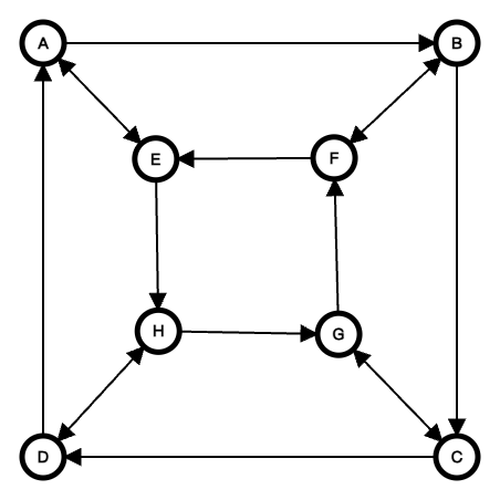
The reason why we choose to find stabilizer codes in the Cayley graph of a dihedral group is because it is a commutative group. We place qudits on the vertices of the Cayley graph. For each qudit, they represent different operations. We define the flip between the vertices in the outer square and the vertices in the inner square to be  $$ \tau $$ , and use  $$ r$$  to represent the rotation of 90 degrees counterclockwise. By following these two rules, we can redenote the vertices, in which  $$ E$$  is set to be the identity element. Thus,  $$ A$$  is  $$ \tau $$ ,  $$ B$$  is  $$ \tau r$$ ,  $$ C$$  is  $$ \tau r^2$$ ,  $$ D$$  is  $$ \tau r^3$$ ,  $$ E$$  is  $$ e$$ ,  $$ H$$  is  $$ r$$ ,  $$ G$$  is  $$ r^2$$ , and  $$ F$$  is  $$ r^3$$ .

Firstly, we choose a stabilizer, in which  $$ X_4$$  is applied on the vertex  $$ \tau $$  and  $$ Z_4$$  is applied on the vertex  $$ e$$ . We denote this stabilizer as

Our purpose is to find a vector  $$ \left(\begin{array}{c}m\\ n\end{array}\right)$$  that commutes with  $$ \left(\begin{array}{c}\tau \\ e\end{array}\right).$$ 

We can apply our formula, thus we can get

$$ \left(\begin{array}{cc}\tau & e\end{array}\right)\times \left(\begin{array}{cc}0& e\\ -e& 0\end{array}\right)\times \left(\begin{array}{c}m\\ n\end{array}\right)=0.$$(12)

Through basic calculation, we can get

$$ \left(\begin{array}{cc}-e& \tau \end{array}\right)\times \left(\begin{array}{c}m\\ n\end{array}\right)=0.$$(13)

Then,

$$ -em+\tau n=0.$$(14)

The relationship between  $$ m$$  and  $$ n$$  is

$$ \tau n=m$$(15)

In this case, it is easy to notice that there are multiple solutions for this equation. We can consider different cases. Here are some possible cases:

6. When  $$ n=\tau $$ ,  $$ m=e$$ .  $$ \left(\begin{array}{c}m\\ n\end{array}\right)=\left(\begin{array}{c}e\\ \tau \end{array}\right)$$ . In this case, the new stabilizer that commutes with the original stabilizer  $$ \left(\begin{array}{cc}\tau & e\end{array}\right)$$ is that  $$ X_4$$  is applied to the vertex  $$ \tau $$  and  $$ Z_4$$  is applied to the vertex  $$ e$$ . Therefore, the stabilizer codes are the combination of  $$ \left(\begin{array}{c}\tau \\ e\end{array}\right)$$  and  $$ \left(\begin{array}{c}e\\ \tau \end{array}\right)$$ .

7. When  $$ n=r$$ ,  $$ m=\tau r$$ .  $$ \left(\begin{array}{c}m\\ n\end{array}\right)=\left(\begin{array}{c}\tau r\\ r\end{array}\right).$$  In this case, the new stabilizer that commutes with the original stabilizer  $$ \left(\begin{array}{cc}\tau & e\end{array}\right)$$  is that  $$ X_4$$  is in  $$ \tau r$$  and  $$ Z_4$$  is in  $$ r$$ . Therefore, the stabilizer codes are the combination of  $$ \left(\begin{array}{c}\tau \\ e\end{array}\right)$$  and  $$ \left(\begin{array}{c}\tau r\\ r\end{array}\right)$$ .

8. When  $$ n=r^2$$ ,  $$ m=\tau r^2$$ .  $$ \left(\begin{array}{c}m\\ n\end{array}\right)=\left(\begin{array}{c}\tau r^2\\ r^2\end{array}\right).$$  In this case, the new stabilizer that commutes with the original stabilizer  $$ \left(\begin{array}{cc}\tau & e\end{array}\right)$$  is that  $$ X_4$$  is in  $$ \tau r^2$$  and  $$ Z_4$$  is in  $$ r^2$$ . Therefore, the stabilizer codes are the combination of  $$ \left(\begin{array}{c}\tau \\ e\end{array}\right)$$  and  $$ \left(\begin{array}{c}\tau r^2\\ r^2\end{array}\right)$$ .

9. Also, we can have some more complicated cases. For example, when  $$ n=r+r^2$$ ,  $$ m=\tau r+\tau r^2$$ .  $$ \left(\begin{array}{c}m\\ n\end{array}\right)=\left(\begin{array}{c}\tau r+\tau r^2\\ r+r^2\end{array}\right).$$ 

Note that when we find stabilizer codes through this way, we can continue to find another one by using the one we just get. For example, for Case 1, we have already got  $$ \left(\begin{array}{c}m\\ n\end{array}\right)=\left(\begin{array}{c}\tau \\ e\end{array}\right)$$ . Therefore, we multiply  $$ \left(\begin{array}{cc}m& n\end{array}\right)$$  with a new stabilizer, denoted by  $$ \left(\begin{array}{c}x\\ y\end{array}\right)$$ . Then we set the  $$ \left(\begin{array}{cc}m& n\end{array}\right)\times \left(\begin{array}{c}x\\ y\end{array}\right)=0$$ , so we can find the value of  $$ \left(\begin{array}{c}x\\ y\end{array}\right)$$ . At this situation, our new stabilizers are the combination of the original given stabilizer  $$ \left(\begin{array}{c}\tau \\ e\end{array}\right)$$ ,  $$ \left(\begin{array}{c}m\\ n\end{array}\right)$$ , and  $$ \left(\begin{array}{c}x\\ y\end{array}\right)$$ . However, through doing calculations, we can get a series of stabilizers for each case. The conditions will be more serious, so eventually the stabilizers will be too complicated to be worth calculating. At that time, we can terminate the process. Ultimately, we can combine the stabilizers to form stabilizer codes.

Therefore, by continuing calculating and finding various solutions, we can get different kinds of stabilizer codes and all of them can be clearly presented on Cayley graph.

7. Conclusion & further exploration

In conclusion, based on existing information of quantum computing and abstract algebra, we have devised an innovative method to find a stabilizer codes to solve our the problem of quantum errors. Specifically, we use a mathematical way to write the common way to find stabilizer codes and find that the methods can be extended to find stabilizer codes on a more complicated group or graph. We also give an example of how to use this method to find a stabilizer group on a dihedral graph  $$ D_4$$ . This approach enables the identification of various stabilizer codes.

The further exploration is to develop a program on computer or to find a mathematical way to compare codes found through this methods among themselves and with existing stabilizer codes, thus contributing to the development of quantum computing.

References

[1]. Andrew Steane. Quantum computing. Reports on Progress in Physics, 61(2):117, 1998.
[2]. David P DiVincenzo and Daniel Loss. Quantum computers and quantum coherence. Journal of Magnetism and Magnetic Materials, 200(1-3):202–218, 1999.
[3]. Andrew M Steane. Error correcting codes in quantum theory. Physical Review Letters, 77(5):793, 1996.
[4]. A Robert Calderbank and Peter W Shor. Good quantum error-correcting codes exist. Physical Review A, 54(2):1098, 1996.
[5]. Andrew Steane. Multiple-particle interference and quantum error correction. Proceedings of the Royal Society of London. Series A: Mathematical, Physical and Engineering Sciences, 452(1954):2551–2577, 1996.
[6]. Andrew M Steane. Simple quantum error-correcting codes. Physical Review A, 54(6):4741, 1996.
[7]. Lucio Piccirillo. Introduction to the Maths and Physics of Quantum Mechanics. CRC Press, 2023.
[8]. Mike Krebs and Anthony Shaheen. Expander families and Cayley graphs: a beginner’s guide. Oxford University Press, 2011.
[9]. Ivan Djordjevic. Quantum information processing and quantum error correction: an engineering approach. Academic press, 2012.
[10]. James C Robinson. An introduction to functional analysis. Cambridge University Press, 2020.
[11]. Jeongwan Haah. Algebraic methods for quantum codes on lattices. arXiv preprint arXiv: 1607. 01387, 2016.
[12]. Gerhard Rosenberger, Annika Schürenberg, and Leonard Wienke. Abstract Algebra: With Applications to Galois Theory, Algebraic Geometry, Representation Theory and Cryptography. Walter de Gruyter GmbH & Co KG, 2024.
[13]. Weisheng Qiu. Group representation theory. Higher Education Press, 2011.
[14]. Mark J DeBonis. Fundamentals of Abstract Algebra. CRC Press, 2024.
[15]. Steven H Simon. Topological quantum: Lecture notes and proto-book. Unpublished prototype. [online] Available at: http://www-thphys. physics. ox. ac. uk/people/SteveSimon, 26:35, 2020.
[16]. Volker Diekert, Manfred Kufleitner, Gerhard Rosenberger, and Ulrich Hertrampf. Elements of Discrete Mathematics: Numbers and Counting, Groups, Graphs, Orders and Lattices. Walter de Gruyter GmbH & Co KG, 2023.
Cite this article
Gui,Y. (2025). Stabilizer Codes on a Cayley Graph. Advances in Operation Research and Production Management,4(1),79-91.
Data availability
The datasets used and/or analyzed during the current study will be available from the authors upon reasonable request.
Disclaimer/Publisher's Note
The statements, opinions and data contained in all publications are solely those of the individual author(s) and contributor(s) and not of EWA Publishing and/or the editor(s). EWA Publishing and/or the editor(s) disclaim responsibility for any injury to people or property resulting from any ideas, methods, instructions or products referred to in the content.
About volume
Journal:Advances in Operation Research and Production Management
© 2024 by the author(s). Licensee EWA Publishing, Oxford, UK. This article is an open access article distributed under the terms and
conditions of the Creative Commons Attribution (CC BY) license. Authors who
publish this series agree to the following terms:
1. Authors retain copyright and grant the series right of first publication with the work simultaneously licensed under a Creative Commons
Attribution License that allows others to share the work with an acknowledgment of the work's authorship and initial publication in this
series.
2. Authors are able to enter into separate, additional contractual arrangements for the non-exclusive distribution of the series's published
version of the work (e.g., post it to an institutional repository or publish it in a book), with an acknowledgment of its initial
publication in this series.
3. Authors are permitted and encouraged to post their work online (e.g., in institutional repositories or on their website) prior to and
during the submission process, as it can lead to productive exchanges, as well as earlier and greater citation of published work (See
Open access policy for details).