1. Introduction

Suppose  $$ \text{P(z)=}{\text{z}}^{\text{n}}\text{+}{\text{a}}_{\text{n-1}}{\text{z}}^{\text{n-1}}\text{+}{\text{a}}_{\text{0}}$$  be a monic polynomial of degree  $$ \text{n}$$ . From Terence Tao’s blog [1], we know we can create a function  $$ \text{P(}\text{t,z}\text{)}$$  of two variables with the given initial data  $$ \text{P(}\text{0,z}\text{)=P(z)}$$  for which

${\mathrm{\partial }}_{t}P(t,z)={\mathrm{\partial }}_{zz}P(t,z)$(1)

where we evolve  $$ \text{P}$$  with respect to time by heat flow. On the space of polynomials of degree at most  $$ \text{n}$$ , the operator  $$ {\text{∂}}_{\text{zz}}$$  is nilpotent, and we can solve this equation explicitly both forwards and backwards in time by the Taylor series. And there is a class of polynomials called orthogonal polynomials, among them we choose Hermite polynomials and apply the deformation operation on them both on normal and matrix polynomials.

2. Preliminaries: properties of analytic functions

An analytic function (or holomorphic function) is a complex function that can be represented by a convergent power series in some neighborhood of every point in its domain. Formally, a function  $$ \text{f(z)}$$  is analytic at a point  $$ {\text{z}}_{\text{0}}$$  if it can be written as

$f(z)={\sum }_{n=0}^{\mathrm{\infty }}{a}_n(z-z_0{)}^n$(2)

where  $$ {\text{a}}_{\text{n}}$$  are complex coefficients, and the series converges within a certain radius around  $$ {\text{z}}_{\text{0}}$$ . The key properties of analytic functions are

•Differentiability: Analytic functions are infinitely differentiable in their domain.

• Power Series Representation: If a function is analytic, it has a Taylor series expansion around any point in its domain, converging to the function in some neighborhood.

• Cauchy-Riemann Equations: For  $$ \text{f(z)=u(}\text{x,y}\text{)+iv(}\text{x,y}\text{)}$$ ,  $$ \text{f}$$  is analytic if  $$ \text{u}$$  and  $$ \text{v}$$  satisfy the Cauchy-Riemann equations:

$\frac{\mathrm{\partial }u}{\mathrm{\partial }x}=\frac{\mathrm{\partial }v}{\mathrm{\partial }y}and\frac{\mathrm{\partial }u}{\mathrm{\partial }y}=-\frac{\mathrm{\partial }v}{\mathrm{\partial }x}$(3)

• Isolated Zeros: If  $$ \text{f(z)}$$  is not identically zero, its zeros are isolated.

• Uniqueness Theorem: If two analytic functions agree on a set with an accumulation point, they are identical throughout their domain.

In this work, we will deal with zeroes of entire functions. One of the main results in this context is the Fundamental Theorem of Algebra. Next, we describe the necessary steps for its proof:

Theorem 2.1 (Liouville’s Theorem). If  $$ \text{f(z)}$$  is entire (analytic everywhere in  $$ \text{C}$$ ) and bounded, then  $$ \text{f(z)}$$  is constant.

Proof. Suppose  $$ \text{f(z)}$$  is entire and bounded by some constant  $$ \text{M}$$ , so  $$ \text{|f(z)|≤M}$$  for all  $$ \text{z∈}\text{C}$$ . By Cauchy’s estimates, we have:

$\mathrm{\mid }{\int }^{(n)}(0)\mathrm{\mid }\le \frac{n!M}{R^n}$(4)

Taking  $$ \text{R→∞}$$ ,  $$ {\text{f}}^{\text{(n)}}\text{(}\text{0)=}\text{0}$$  for all  $$ \text{n≥1}$$ , implying that  $$ \text{f(z)=}\text{f(}\text{0)}$$ . Hence,  $$ \text{f}$$  is constant.

Theorem 2.2 (Fundamental Theorem of Algebra). Every non-constant polynomial  $$ \text{P(z)}$$  with complex coefficients has at least one root in  $$ \text{C}$$ .

Proof. Assume for contradiction that  $$ \text{P(z)}$$  has no roots in  $$ \text{C}$$ . Define  $$ \text{f(z)=}\frac{\text{1}}{\text{P(z)}}$$ , which is entire and bounded as  $$ \text{|P(z)|→∞}$$  as  $$ \text{|z|→∞}$$ . By Liouville’s Theorem,  $$ \text{f(z)}$$  is constant, which implies  $$ \text{P(z)}$$  is constant—a contradiction.

3. Polynomial deformation and root motion

Consider a polynomial  $$ \text{P(z) = }{\text{a}}_{\text{n}}\text{(z-}{\text{z}}_{\text{1}}\text{)(z-}{\text{z}}_{\text{2}}\text{)…(z-}{\text{z}}_{\text{n}}\text{)}$$  with real coefficients, and deform it as  $$ \text{P(}\text{z,t}\text{)}$$  such that  $$ \text{P(z,}\text{0)=}\text{P(z)}$$ . Let the deformation satisfy

${\mathrm{\partial }}_{t}P(t,z)={\mathrm{\partial }}_{zz}P(t,z)$(5)

where  $$ \text{t≥0}$$ .

We follow the steps in Terecene’s Blog [1].

Example 3.1. (Quadratic Polynomial)

Take  $$ \text{P(z)=}{\text{z}}^{\text{2}}\text{+}\text{bz+c}\text{.}$$  A deformation is given by

$P(z,t)=z^2+bz+c+2t$(6)

The roots of  $$ \text{P(}\text{z,t}\text{)}$$  depend on  $$ \text{t}$$ :

• For  $$ \text{t<}\frac{{\text{b}}^{\text{2}}\text{-4c}}{\text{8}}$$  , the roots are real and approach each other as t increases.

• When  $$ \text{t=}\frac{{\text{b}}^{\text{2}}\text{-4c}}{\text{8}}$$ , the roots collide.

• For  $$ \text{t>}\frac{{\text{b}}^{\text{2}}\text{-4c}}{\text{8}}$$ , the roots become complex and move vertically in the complex plane.

3.1. Heat flow polynomials and their roots motion

Theorem 3.2 (explicit expression for heat deformation). An explicit expression for the heat flow deformation equation is:

$P(t,z)={\sum }_{j=0}^{\mathrm{\infty }}\frac{t^j}{j!}{\mathrm{\partial }}_{zz}^{j}P(z)$(7)

Proof. The deformation conditions are:

${\mathrm{\partial }}_{t}P(t,z)={\mathrm{\partial }}_{zz}P(t,z)$(8)

with the initial condition  $$ \text{P(}\text{0,z}\text{)=P(z)}$$ . Applying the Taylor series expansion of  $$ \text{P(}\text{t,z}\text{)}$$  with respect to  $$ \text{t}$$  around  $$ \text{t=0}$$ , we obtained the following.

$P(t,z)={\sum }_{j=0}^{\mathrm{\infty }}\frac{(t-0{)}^j}{j!}{\mathrm{\partial }}_t^{j}P(0,z)$(9)

Inserting the knowing conditions, we get:

$P(t,z)={\sum }_{j=0}^{\mathrm{\infty }}\frac{t^j}{j!}{\mathrm{\partial }}_{zz}^{j}P(z)$(10)

as desired.

Starting from  $$ \text{P(t,}{\text{z}}_{\text{i}}\text{(t}\text{))=}\text{0}$$  for each root  $$ {\text{z}}_{\text{i}}\text{(t)}$$ , differentiating with respect to t and using the chain rule and the heat equation gives:

${\mathrm{\partial }}_{zz}P(t,z_i(t))+{\mathrm{\partial }}_t{z}_i(t){\mathrm{\partial }}_{z}P(t,z_i(t))=0$(11)

Theorem 3.3 (Mutual Effects between the real roots). Let  $$ \text{P(}\text{z;t}\text{)}$$  be a heat deformed polynomial with initial condition  $$ \text{P(z;}\text{0)=}\text{P(z)}$$ , where  $$ \text{P(z)}$$  is a polynomial of degree  $$ \text{n}$$ . Let  $$ {\text{z}}_{\text{i}}\text{, }\text{i}\text{=1, ..., n}$$  be the roots of  $$ {\text{P}}_{\text{n}}\text{(}\text{z;t}\text{)}$$ . Then the following evolution equations hold

$\frac{\mathrm{\partial }}{\mathrm{\partial }t}{z}_m(t)=-{\sum }_{i\mathrm{\ne }m}\frac{2}{z_m-z_i},m=1,\dots ,n$(12)

Proof. Using the fundamental theorem of Algebra, we can write the deformed polynomial as follows:

$P(z,t)=(z-z_1)(z-z_2)\cdots (z-z_n)$(13)

Take its first partial derivative with respect to z using product rule, we get:

$\begin{array}{cc}\frac{\mathrm{\partial }P}{\mathrm{\partial }z}& =(z-z_1)\mathrm{\prime }(z-z_2)\cdots (z-z_n)+(z-z_1)(z-z_2)\mathrm{\prime }\cdots (z-z_n)+\cdots +(z-z_1)(z-z_2)\cdots (z-z_n)\mathrm{\prime }\\ & =1\cdot (z-z_2)(z-z_3)\cdots (z-z_n)+\cdots +(z-z_1)(z-z_2)\cdots (z-z_{n-1})\cdot 1\\ & ={\sum }_{i=1}^n{\prod }_{k\mathrm{\ne }i}(z-z_k)\mathrm{.}\end{array}$(14)

Similarly, its second partial derivative with respect to z is:

$\frac{{\mathrm{\partial }}^{2}P}{\mathrm{\partial }{z}^2}={\sum }_{i=1}^n{\sum }_{j\mathrm{\ne }i}{\prod }_{k\mathrm{\ne }i,k\mathrm{\ne }j}(z-z_k)$(15)

Next, we insert  $$ {\text{z}}_{\text{m}}\text{→z}$$ . For the first partial derivative, we have the summation of n terms indexed by  $$ \text{i}$$ :

${\prod }_{k\mathrm{\ne }i}(z_m-z_k)$(16)

And we have four cases:

(1) If  $$ \text{i≠m}\text{,}\prod _{\text{k≠i}}\text{(}{\text{z}}_{\text{m}}\text{-}{\text{z}}_{\text{k}}\text{)=0}$$ , as it contains factor  $$ \text{(}{\text{z}}_{\text{m}}\text{-}{\text{z}}_{\text{m}}\text{)}$$ .

(2) If  $$ \text{i}\text{=m,}\prod _{\text{k≠i}}\text{(}{\text{z}}_{\text{m}}\text{-}{\text{z}}_{\text{k}}\text{)=0}$$  survives as it drops out  $$ \text{(}{\text{z}}_{\text{m}}\text{-}{\text{z}}_{\text{m}}\text{)}$$ .

Thus,

$\frac{\mathrm{\partial }}{\mathrm{\partial }z}P(z_m)={\prod }_{k\mathrm{\ne }m}(z_m-z_k)$(17)

Continue with the second partial derivative

$\frac{{\mathrm{\partial }}^2}{\mathrm{\partial }{z}^2}P(z_m)$(18)

Here we have the sum of  $$ \text{n⋅(n-1)\hspace{0.17em}}\text{i,j}$$ -indexed terms:

${\prod }_{k\mathrm{\ne }i,j}(z_m-z_k)$(19)

From combinatorial point of view, each term

${\prod }_{k\mathrm{\ne }i,j}(z_m-z_k)$(20)

is obtained by dropping out 2 chosen components  $$ \text{(}{\text{z}}_{\text{m}}\text{-}{\text{z}}_{\text{i}}\text{),(}{\text{z}}_{\text{m}}\text{-}{\text{z}}_{\text{j}}\text{).}$$ 

(3) If  $$ \text{i}\text{=m}$$  or  $$ \text{j=m}$$ ,  $$ \prod _{\text{k≠}\text{i,j}}\text{(}{\text{z}}_{\text{m}}\text{-}{\text{z}}_{\text{k}}\text{)}$$  survives as the zero term  $$ \text{(}{\text{z}}_{\text{m}}\text{-}{\text{z}}_{\text{m}}\text{)}$$  is dropped.

(4) If  $$ \text{i≠m}$$  and  $$ \text{j≠m}$$ ,  $$ \prod _{\text{k≠}\text{i,j}}\text{(}{\text{z}}_{\text{m}}\text{-}{\text{z}}_{\text{k}}\text{)=0}$$ .

Thus,

$\frac{{\mathrm{\partial }}^2}{\mathrm{\partial }{z}^2}P(z_m)={\sum }_{i\mathrm{\ne }m}{\prod }_{k\mathrm{\ne }i,m}(z_m-z_k)+{\sum }_{j\mathrm{\ne }m}{\prod }_{k\mathrm{\ne }m,j}(z_m-z_k)=2{\sum }_{i\mathrm{\ne }m}{\prod }_{k\mathrm{\ne }i,m}(z_m-z_k)$(21)

At the beginning of this subsection, we used the chain rule and deformation assumptions to get the following implicit differentiation:

${\mathrm{\partial }}_{zz}P(t,z_m(t))+{\mathrm{\partial }}_t{z}_m(t){\mathrm{\partial }}_{z}P(t,z_m(t))=0$(22)

Therefore,

$\frac{\mathrm{\partial }}{\mathrm{\partial }t}{z}_m=-\frac{\frac{{\mathrm{\partial }}^2}{\mathrm{\partial }{z}^2}P(z_m)}{\frac{\mathrm{\partial }}{\mathrm{\partial }z}P(z_m)}=-2\frac{{\sum }_{i\mathrm{\ne }m}{\prod }_{k\mathrm{\ne }i,m}(z_m-z_k)}{{\prod }_{k\mathrm{\ne }m}(z_m-z_k)}=-{\sum }_{i\mathrm{\ne }m}\frac{2}{z_m-z_i}$(23)

Corollary 3.4 (Attraction of real roots). Suppose there exist  $$ \text{a,b}\text{>0}$$  such that for any  $$ \text{t∈[}\text{a,b}\text{]}$$ , the functions  $$ {\text{z}}_{\text{m}}\text{(t)}$$  are the simple real roots of the polynomial:

$P(t,z)={\sum }_{j=0}^{\mathrm{\infty }}\frac{t^j}{j!}{\mathrm{\partial }}_{zz}^{j}P(z)$(24)

then each term  $$ \frac{\text{2}}{{\text{z}}_{\text{m}}\text{-}{\text{z}}_{\text{i}}}$$  represents a first-order attraction in the dynamics between  $$ {\text{z}}_{\text{i}}$$  and  $$ {\text{z}}_{\text{m}}$$ . Proof. From Theorem 4, we know

$\frac{\mathrm{\partial }}{\mathrm{\partial }t}{z}_m={\sum }_{i\mathrm{\ne }m}\frac{2}{z_i-z_m}$(25)

Consider the case where we have only two roots,  $$ {\text{z}}_{\text{m}}$$  and  $$ {\text{z}}_{\text{i}}$$ . In this scenario,

$\frac{\mathrm{\partial }}{\mathrm{\partial }{z}_m}=\frac{2}{z_i-z_m}\mathrm{\ne }0$(26)

If  $$ {{\text{z}}_{\text{i}}\text{>z}}_{\text{m}}$$ , then  $$ \frac{\text{∂}}{\text{∂t}}{\text{z}}_{\text{m}}\text{>0}$$ . Conversely,  $$ \frac{\text{∂}}{\text{∂t}}{\text{z}}_{\text{i}}\text{=}\frac{\text{2}}{{\text{z}}_{\text{m-}{\text{z}}_{\text{i}}}}\text{<0}$$ . Thus, as  $$ \text{t}$$  increases,  $$ {\text{z}}_{\text{m}}$$  will increase, and  $$ {\text{z}}_{\text{i}}$$  will decrease. Consequently, they exhibit attraction-like behavior. The same reasoning applies if  $$ {{\text{z}}_{\text{i}}\text{<z}}_{\text{m}}$$ , as the indices can be exchanged symmetrically.

In the general case, assume we have at least two distinct simple real roots. Define

$z_s=max(z_i),z_t=min(z_i),with{z}_s>z_t$(27)

For any  $$ \text{j≠}\text{s,t}$$ , it holds that  $$ \frac{\text{2}}{{\text{z}}_{\text{j-}}{\text{z}}_{\text{s}}}\text{<0 and }\frac{\text{2}}{{\text{z}}_{\text{j-}}{\text{z}}_{\text{t}}}\text{>0}$$ . So  $$ \frac{\text{∂}}{\text{∂t}}{\text{z}}_{\text{s}}\text{<0 and }\frac{\text{∂}}{\text{∂t}}{\text{z}}_{\text{t}}\text{>0}$$ . From the above observation,  $$ {\text{z}}_{\text{s}}$$  and  $$ {\text{z}}_{\text{t}}$$  exhibit attraction-like behavior as  $$ \text{t}$$  increases.

Moreover, if we remove either  $$ {\text{z}}_{\text{s}}$$  or  $$ {\text{z}}_{\text{t}}$$  from consideration, we can repeat the process with the remaining roots to identify a new attraction relationship between two real roots. This iterative process ensures that all real roots are eventually paired in attraction-like relationships

3.2. Plot of root movement

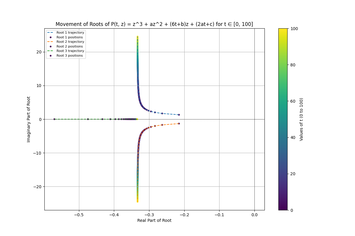
Figure 1 shows the movement of the roots of  $$ \text{P(}\text{z,t}\text{)=}{\text{z}}^{\text{2}}\text{+bz+c+2t}$$ , as  $$ \text{t}$$  varies.

3.3. Polynomial deformations and root movement

Using the heat flow equation, we explored how polynomial roots evolve under deformation. Three examples were analyzed and visualized:

3.3.1. Example 1: a quadratic polynomial

For  $$ \text{P(}\text{t,z}\text{)=}{\text{z}}^{\text{3}}\text{+}{\text{z}}^{\text{2}}\text{+(6t+}\text{2)z}\text{+(1+2t)}$$ , roots transitioned from real to complex as t increased. The trajectories were smooth, with collision points determined analytically.

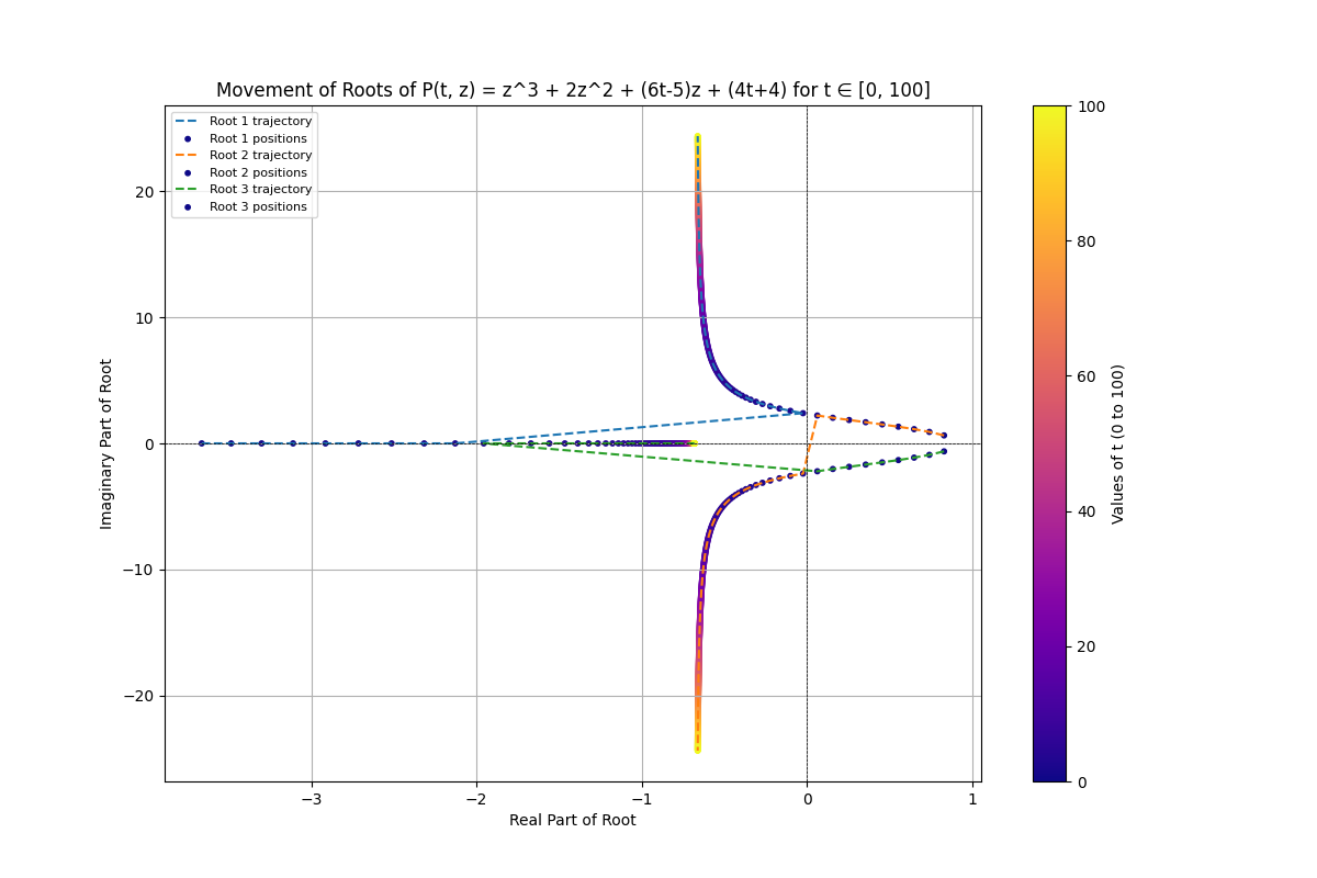
3.3.2. Example 2: a cubic polynomial

For  $$ \text{P(}\text{t,z}\text{)=}{\text{z}}^{\text{3}}\text{+2}{\text{z}}^{\text{2}}\text{+(6t-}\text{5)z}\text{+(4t+4)}$$ , root interactions led to sharp transitions and bifurcations in trajectories.

3.3.3. Example 3: extreme coefficients

The extreme case  $$ \text{P(}\text{t,z}\text{)=}{\text{z}}^{\text{3}}\text{+5}{\text{z}}^{\text{2}}\text{+(6t-}\text{20)z}\text{+(4t+10)}$$  revealed dramatic root behaviors, with visible jumps and deviations from smooth trajectories.

3.4. Conclusion

The dynamic behavior of polynomial roots under heat flow provided intuition for complex deformations, while orthogonal polynomials showcased the depth of classical mathematical structures. Future work may involve extending these techniques to higher-degree polynomials or exploring numerical stability in root motion algorithms.

4. Exploring heat flow, orthogonal polynomials, and deformations of polynomials

4.1. Orthogonal polynomials: definitions and classical families. a weight function

 $$ \text{w(x)}$$  on  $$ \text{[}\text{a,b}\text{]}$$  is a nonegative function with finite moments of every order:

${\int }_a^b{x}^{n}w(x)dx<\mathrm{\infty }$(28)

Asequence of orhtogonal polynomials  $$ \text{P(n)}$$  satisfies:

${\int }_a^b{P}_n(x)P_m(x)w(x)dx=0forn\mathrm{\ne }m$(29)

Note that functions  $$ \text{w(x)>0}$$  ensure convergence of the integral and define classical families of orthogonal polynomials. The Classical Families are (Figure 2):

•Hermite Polynomials: Orthogonal on  $$ \text{(-}\text{∞,∞}\text{)}$$  with  $$ \text{w(x)=}{\text{e}}^{\text{-}{\text{x}}^{\text{2}}}$$ .

• Laguerre Polynomials: Orthogonal on  $$ \text{[}\text{0,∞}\text{)}$$  with $$ \text{ w(x)=}{\text{e}}^{\text{-x}}{\text{x}}^{\text{α}}\text{,\hspace{0.17em}α>-1}$$ .

• Chebyshev Polynomials: Orthogonal on  $$ \text{[-1,1]}$$  with weight functions depending on the family  $$ \text{(}{\text{T}}_{\text{n}}\text{ or }{\text{U}}_{\text{n}}\text{)}$$ .

4.2. Three-term recurrence relation and some consequences

Theorem 4.1. (Three-Term Recurrence Relation) Orthogonal polynomials  $$ {\text{p}}_{\text{n}}$$  satisfy

$x{p}_n(x)=a_{n+1}{p}_{n+1}(x)+b_n{p}_n(x)+c_n{p}_{n-1}(x),(n>0)$(30)

${\text{xp}}_0{\text{(x)=a}}_0{\text{p}}_1{\text{(x)+b}}_0{\text{p}}_0\text{(x)}$(31)

with  $$ {\text{a}}_{\text{n}}\text{,}{\text{b}}_{\text{n}}\text{,}{\text{c}}_{\text{n}}$$  real constants and  $$ {\text{a}}_{\text{n}}{\text{c}}_{\text{n}\text{+1}}\text{>0}$$ . Also,

$a_n=\frac{k_n}{k_{n+1}},\frac{c_{n+1}}{h_{n+1}}=\frac{a_n}{h_n}$(32)

Remarks:

(1) For orthonormal polynomials, the recurrence relation becomes:

$x{\pi }_n(x)=a_{n+1}{\pi }_{n+1}(x)+b_n{\pi }_n(x)+a_{n-1}{\pi }_{n-1}(x),(n>0),$(33)

$x{\pi }_0(x)=a_0{\pi }_1(x)+b_0{\pi }_0(x),$(34)

(2) If the orthogonality measure is even  $$ \text{(μ(-}\text{x)=}\text{μ(x))}$$ , then  $$ {\text{p}}_{\text{n}}\text{(-}\text{x)=}\text{(-1}{\text{)}}^{\text{n}}{\text{p}}_{\text{n}}\text{(x)}$$ , and  $$ {\text{b}}_{\text{n}}\text{=0.}$$  Examples include Legendre and Hermite polynomials.

(3) The recurrence relation determines the polynomials  $$ {\text{p}}_{\text{n}}\text{(x)}$$  uniquely up to a constant factor (depending on the normalization).

(4) The orthogonality measure for a system of orthogonal polynomials may not be unique.

(5) If the orthogonality measure has bounded support, then it is unique. (Figure 3)

4.3. Zeros of orthogonal polynomials

Let  $$ {\text{p}}_{\text{n}}\text{(}\text{x}\text{)}$$  be an orthogonal polynomial of degree  $$ \text{n}$$ . If  $$ \text{μ}$$  has support within the interval  $$ \text{[}\text{a}\text{,}\text{b}\text{]}$$ , then:

(1)  $$ {\text{p}}_{\text{n}}\text{(x)}$$  has  $$ \text{n}$$  distinct zeros in  $$ \text{(}\text{a,b}\text{)}$$ .

(2) The zeros of  $$ {\text{p}}_{\text{n}}\text{(x)}$$  and  $$ {\text{p}}_{\text{n-1}}\text{(x)}$$  alternate.

4.4. Hermite polynomials

Definition 4.2. The Hermite polynomials  $$ {\text{H}}_{\text{n}}\text{(}\text{x}\text{)}$$  are a classical family of orthogonal polynomials defined by the Rodrigues’ formula:

$H_n(x)=(-1{)}^n{e}^{x^2}\frac{d^n}{d{x}^n}(e^{-x^2}),n=0,1,2,\dots$(35)

Proposition 4.3. (Orthogonality) Hermite polynomials are orthogonal on the interval  $$ \text{(-}\text{∞,∞}\text{)}$$  with respect to the weight function  $$ \text{w}\text{(}\text{x}\text{)=}{\text{e}}^{\text{-}{\text{x}}^{\text{2}}}$$  . The orthogonality condition is given by:

${\int }_{-\mathrm{\infty }}^{\mathrm{\infty }}{H}_n(x)H_m(x)e^{-x^2}dx=\sqrt[]{\pi }{2}^n\eta !{\delta }_{nm}$(36)

where  $$ {\text{δ}}_{\text{nm}}$$  is the Kronecker delta.

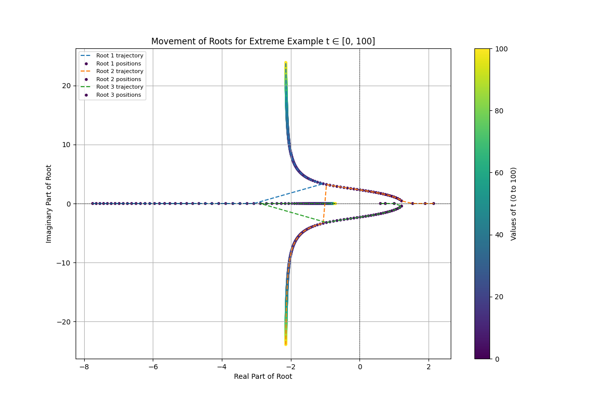
Figure 4 shows the movement of the Roots for Example 3 as mentioned in 3.3.3.

Proposition 4.4. (Recurrence Relation) The Hermite polynomials satisfy the following recurrence relation:

$H_{n+1}(x)=2x{H}_n(x)-2n{H}_{n-1}(x),n\ge 1,$(37)

with initial conditions:  $$ {\text{H}}_{\text{0}}\text{(}\text{x}\text{)=1}$$ ,  $$ {\text{H}}_{\text{1}}\text{(}\text{x}\text{)=2}\text{x}$$ 

Proposition 4.5. (Generating Function) The generating function for Hermite polynomials is:

${\sum }_{n=0}^{\mathrm{\infty }}\frac{t^n}{n!}{H}_n(x)=e^{2xt-t^2}$(38)

Proposition 4.6. (Other key properties)

• Symmetry:

$H_n(-x)=(-1{)}^n{H}_n(x)$(39)

• Differential Equation: Hermite polynomials satisfy the second-order differential equation:

$H_n^{\mathrm{\prime }\mathrm{\prime }}(x)-2x{H}_n^{\mathrm{\prime }}(x)+2n{H}_n(x)=0$(40)

• Explicit Formula:

$H_n(x)={\sum }_{k=0}^{[n\mathrm{/}2]}\frac{(-1{)}^{k}n!}{k!(n-2k)!}(2x{)}^{n-2k}$(41)

• First derivative:

$H_n^{\mathrm{\prime }}(x)=2n{H}_{n-1}(x)$(42)

5. Deformation of hermite polynomial

5.1. Original hermite polynomials

The Hermite polynomials  $$ {\text{H}}_{\text{n}}\text{(x)}$$  for  $$ \text{n=1,2,3}$$  are shown in Figure 5, with their polynomial expressions displayed.

5.2. Formula for Hermite polynomial after deformation

Theorem 5.1. The formula for Hermite polynomial of degree  $$ \text{n}$$  after deformation is the following

$H_n(z,t)={\sum }_{j=0}^{\mathrm{\infty }}\frac{t^j}{j!}{2}^{2j}\frac{n!}{(n-2j)!}{H}_{n-2j}(z)$(43)

Proof. We know the original formula for deformation is

$H_n(z,t)={\sum }_{j=0}^{\mathrm{\infty }}\frac{t^j}{j!}{\mathrm{\partial }}_{zz}{H}_n(z)$(44)

By the property of Hermite polynomial we know

$H_n^{\mathrm{\prime }}(z)=2n{H}_{n-1}(z)\Rightarrow H_n^{\mathrm{\prime }\mathrm{\prime }}(z)=4(n-1)n{H}_{n-2}(z)$(45)

So we can claim that

${\mathrm{\partial }}_{zz}^j{H}_n(z)=4^j\frac{n!}{(n-2j)!}{H}_{n-2j}(z)$(46)

We can prove it by induction, tha basic case we have shown before. So suppose it is true for  $$ \text{j}\text{=}\text{k}$$ . Then

${\mathrm{\partial }}_{zz}^{j+1}{H}_n(z)={\mathrm{\partial }}_{zz}({\mathrm{\partial }}_{zz}^j{H}_n(z))$(47)

By induction hypothesis we have

$\begin{array}{cc}& {\mathrm{\partial }}_{zz}(4^j\frac{n!}{(n-2j)!}{H}_{n-2j}(z))\\ & =4^j\frac{n!}{(n-2j)!}{\mathrm{\partial }}_{zz}{H}_{n-2j}(z)\\ & =4^j\frac{n!}{(n-2j)!}4(n-2j-1)(n-2j)H_{n-2(j+1)}(z)\\ & =4^{j+1}\frac{n!}{(n-2j-2)!(n-2j-1)(n-2j)}(n-2j-1)(n-2j)H_{n-2(j+1)}(z)\\ & =4^{j+1}\frac{n!}{(n-2(j+1))!}{H}_{n-2(j+1)}(z)\mathrm{.}\end{array}$(48)

By induction we have done.

5.3. Deformation even degree Hermite polynomial

By theorem 5.1 every even degree

Hermite polynomial can be written as this following form.

$H_{2s}(z,t)={\sum }_{j=0}^s\frac{t^j}{j!}{2}^{2j}\frac{2s!}{(2s-2j)!}{H}_{2(s-j)}(z)$(49)

To prove the following lemma we need the definition of hypergeometric series and the relation between it and Hermite polynomial.

Definition 5.2. For natural number p and q the hypergeometric series is

$\begin{array}{c}{}_p{F}_q(\begin{array}{c}{a}_1,a_2,\dots ,a_p\\ b_1,b_2,\dots ,b_q\\ \end{array};z)={\sum }_{n=0}^{\mathrm{\infty }}\frac{(a_1{)}_n(a_2{)}_n\cdots (a_p{)}_n}{(b_1{)}_n(b_2{)}_n\cdots (b_q{)}_n}\frac{z^n}{n!},\end{array}$(50)

where the Pochhammer symbol (rising factorial) is

$(a{)}_n=a(a+1)(a+2)\cdots (a+n-1)=\frac{\mathrm{\Gamma }(a+n)}{\mathrm{\Gamma }(a)}$(51)

And  $$ \text{(}\text{a}{\text{)}}_{\text{0}}\text{=1}$$ 

And here is the formula to write Hermite polynomial by hypergeometric series, We won’t prove it here. Formal proof can be found in here: [2]

Theorem 5.3. Give Hermite polynomial of degree  $$ \text{n}$$ .

$H_n(z)=(2z{{)}^n}_2{F}_0(\begin{array}{c}-\frac{n}{2},-\frac{(n-1)}{2}\\ {}_{-}\\ {}_{-}\\ \end{array};-\frac{1}{z^2})$(52)

Lemma 5.4. The following formula for even degree Hermite polynomial is true, Given s, a natural number

$H_{2s}(z,t)={\sum }_{j=0}^s\frac{t^j}{j!}\frac{(2s)!}{(2s-2j)!}{2}^{2s}{\sum }_{k=0}^{s-j}\frac{(-s+j{)}_k(-s+j+\frac{1}{2}{)}_k}{k!}(-1{)}^k{z}^{-2k+2s-2j}$(53)

Where

$(x{)}_j=x(x+1)\dots (x+j-1)$(54)

Proof. By theorem 5.3 we know take  $$ \text{s}$$ ,  $$ \text{j}$$  natural number,  $$ \text{j}\text{<}\text{s}$$ 

$\begin{array}{cc}{H}_{2(s-j)}(z)& =(2z{)}_2^{2(s-j)}{F}_0(\begin{array}{c}-s+j,-s+j+\frac{1}{2}\\ -\\ \end{array};-\frac{1}{z^2})\\ & =(2z{)}^{2(s-j)}{\sum }_k^{\mathrm{\infty }}\frac{(-s+j{)}_k(-s+j+\frac{1}{2}{)}_k}{k!}(-\frac{1}{z^2}{)}^k\end{array}$(55)

Notice that  $$ \text{-}\text{s}\text{+}\text{j}\text{<0}$$ , by the definition of pochhammer symbol we know  $$ \text{(-}\text{s}\text{+}\text{j}{\text{)}}_{\text{k}}\text{=0}$$  for every  $$ \text{k}\text{>}\text{s}\text{-}\text{j}$$ . So we have

$\begin{array}{cc}{H}_{2(s-j)}(z)& =(2z{)}^{2(s-j)}{\sum }_k^{s-j}\frac{(-s+j{)}_k(-s+j+\frac{1}{2}{)}_k}{k!}(-\frac{1}{z^2}{)}^k\\ & =2^{2(s-j)}{z}^{2s-2j}{\sum }_k^{s-j}\frac{(-s+j{)}_k(-s+j+\frac{1}{2}{)}_k}{k!}(-1{)}^k{z}^{-2k}\\ & =2^{2(s-j)}{\sum }_k^{s-j}\frac{(-s+j{)}_k(-s+j+\frac{1}{2}{)}_k}{k!}(-1{)}^k{z}^{-2k+2s-2j}\end{array}$(56)

Recall we know

$H_{2s}(z,t)={\sum }_{j=0}^s\frac{t^j}{j!}{2}^{2j}\frac{2s!}{(2s-2j)!}{H}_{2(s-j)}(z)$(57)

Substitute  $$ {\text{H}}_{\text{2(}\text{s}\text{-}\text{j}\text{)}}\text{(}\text{z}\text{)}$$  term in our formula we have done

From lemma 5.4 we know if we consider  $$ {\text{H}}_{\text{zs}}\text{(}\text{z}\text{,}\text{t}\text{)}$$  as an polynomial of  $$ \text{z}$$  and denote  $$ {\text{a}}^{\text{k}}$$  the

coefficient of  $$ {\text{z}}^{\text{k}}$$  . Then since the degree of  $$ \text{z}$$  is always even,

we know  $$ {\text{a}}_{\text{2}\text{n}\text{+1}}\text{=0}$$  for all  $$ \text{n}\text{∈}\text{N}\text{.}$$ . In the following lemma we will see the coefficient of even term.

Theorem 5.5. Denote  $$ {\text{a}}_{\text{2}\text{n}}$$  coefficient of  $$ {\text{z}}^{\text{2}\text{n}}$$  in the polynomial  $$ {\text{H}}_{\text{2}\text{s}}\text{(}\text{z}\text{,}\text{t}\text{)}$$ , Then

$a_{2n}=4^s(n+1{)}_{s-n}(n+\frac{1}{2}{)}_{s-n}\frac{(4t-1{)}^{s-n}}{(s-n)!}$(58)

Proof. From lemma 5.4 we know

$H_{2s}(z,t)={\sum }_{j=0}^s\frac{t^j}{j!}\frac{(2s)!}{(2s-2j)!}{2}^{2s}{\sum }_{k=0}^{s-j}\frac{(-s+j{)}_k(-s+j+\frac{1}{2}{)}_k}{k!}(-1{)}^k{z}^{-2k+2s-2j}$(59)

Here we denote  $$ \text{2}\text{n}\text{=2(}\text{s}\text{-}\text{j}\text{-}\text{k}\text{)⇒}\text{n}\text{=}\text{s}\text{-}\text{j}\text{-}\text{k}\text{⇒}\text{k}\text{=}\text{s}\text{-}\text{j}\text{-}\text{n}\text{.}$$  For fixed  $$ \text{s}$$ , We know  $$ \text{k}$$  is determined by  $$ \text{j}$$  and  $$ \text{n}$$ . Now we want to study the coefficient of  $$ {\text{z}}^{\text{n}}$$ which means that  $$ \text{n}$$  is also given when we look at the formula of  $$ {\text{a}}_{\text{2}\text{n}}$$ . Thus once we know the value of  $$ \text{k}$$  or  $$ \text{j}$$ , then we know the value of another one. The double sums become a single sum, here we choose  $$ \text{j}$$  as variable. Also notice that  $$ \text{j}\text{+}\text{k}\text{=}\text{s}\text{-}\text{n}\text{.}$$  Thus we have

$\begin{array}{cc}{a}_{2n}& ={\sum }_{j=0}^{s-n}{4}^s\frac{t^j}{j!}\frac{(2s)!}{(2s-2j)!}\frac{(-s+j{)}_{s-n-j}(-s+j+\frac{1}{2}{)}_{s-n-j}}{(s-n-j)!}(-1{)}^{s-n-j}\\ & ={\sum }_{j=0}^{s-n}{4}^j\frac{t^j}{j!(s-n-j)!}(-1{)}^{s-n-j}{4}^{s-j}\frac{(2s)!(-s+j{)}_{s-n-j}(-s+j+\frac{1}{2}{)}_{s-n-j}}{(2s-2j)!}\end{array}$(60)

Notice that

$\begin{array}{cc}(2s-2j)!& =(2s-2j)(2s-2j-1)\dots 21=2^{2s-2j}(s-j)(s-j-\frac{1}{2})\dots 1\frac{1}{2}\\ & =4^{s-j}(s-j)(s-j-1)\dots 21(s-j-\frac{1}{2})(s-j-\frac{3}{2})(s-j-\frac{5}{2})\dots \frac{1}{2}\end{array}$(61)

Also notice that

$\begin{array}{cc}(-s+j{)}_{s-j-n}& =(-s+j)(-s+j+1)\dots (-n-1)\\ & =(-1{)}^{s-j-n}(s-j)\dots (n+1)\end{array}$(62)

For the same reason

$(-s+j+\frac{1}{2}{)}_{s-j-n}=(-1{)}^{s-j-n}(s-j-\frac{1}{2})\cdots (n+\frac{1}{2})$(63)

Combine them together we have

$\frac{(-s+j{)}_{s-n-j}(-s+j+\frac{1}{2}{)}_{s-n-j}}{(2s-2j)!}=\frac{(s-j)\dots (n+1)(s-j-\frac{1}{2})\dots (n+\frac{1}{2})}{4^{s-j}(s-j)(s-j-1)\dots 21(s-j-\frac{1}{2})(s-j-\frac{3}{2})\dots \frac{1}{2}}$(64)

And since  $$ \text{n}\text{=}\text{s}\text{-}\text{j}\text{-}\text{k}\text{<=}\text{s}\text{-}\text{j}\text{.}$$ . If  $$ \text{n}\text{=}\text{s}\text{-}\text{j}\text{⇒}\text{s}\text{-}\text{j}\text{-}\text{n}\text{=0}$$ . By the def of Pochhammer symbol

$\begin{array}{cc}\frac{(-s+j{)}_{s-n-j}(-s+j+\frac{1}{2}{)}_{s-n-j}}{(2s-2j)!}& =\frac{1}{(2n)!}=\frac{1}{4^{n}n!(n-\frac{1}{2})\cdots \frac{1}{2}}\\ & =\frac{1}{4^{s-j}n!(n-\frac{1}{2})\cdots \frac{1}{2}}\end{array}$(65)

Then for  $$ \text{n}\text{=}\text{s}\text{-}\text{j}\text{-}\text{k}\text{<}\text{s}\text{-}\text{j}$$  then we have

$\begin{array}{cc}& \frac{(s-j)\dots (n+1)(s-j-\frac{1}{2})\dots (n+\frac{1}{2})}{4^{s-j}(s-j)(s-j-1)\dots 21(s-j-\frac{1}{2})(s-j-\frac{3}{2})\dots \frac{1}{2}}\\ & =\frac{(s-j)\dots (n+1)(s-j-\frac{1}{2})\dots (n+\frac{1}{2})}{4^{s-j}(s-j)\dots (n+1)n\dots 1(s-j-\frac{1}{2})\dots (n+\frac{1}{2})(n-\frac{1}{2})\dots \frac{1}{2}}\\ & =\frac{1}{4^{s-j}n!(n-\frac{1}{2})\cdots \frac{1}{2}}\end{array}$(66)

So it is true for all proper  $$ \text{n}$$ . Also notice that

$(2s)!=2^{2s}s(s-\frac{1}{2})\cdots \frac{1}{2}=4^{s}s!(s-\frac{1}{2})\cdots \frac{1}{2}$(67)

Putting all together we have

$\begin{array}{cc}& 4^{s-j}\frac{(2s)!(-s+j{)}_{s-n-j}(-s+j+\frac{1}{2}{)}_{s-n-j}}{(2s-2j)!}=4^{s-j}\frac{4^{s}s!(s-\frac{1}{2})\cdots \frac{1}{2}}{4^{s-j}n!(n-\frac{1}{2})\cdots \frac{1}{2}}\\ & =4^s\frac{s!(s-\frac{1}{2})\cdots \frac{1}{2}}{n!(n-\frac{1}{2})\cdots \frac{1}{2}}=4^{s}s(s-1)\cdots (n+1)(s-\frac{1}{2})(s-\frac{3}{2})\cdots (n+\frac{1}{2})\\ & =4^s(n+1{)}_{s-n}(n+\frac{1}{2}{)}_{s-n}\end{array}$(68)

Going back to the original formula for  $$ {\text{a}}_{\text{2}\text{n}}$$ , we have

$\begin{array}{cc}{a}_{2n}& ={\sum }_{j=0}^{s-n}{4}^j\frac{t^j}{j!(s-n-j)!}(-1{)}^{s-n-j}{4}^s(n+1{)}_{s-n}(n+\frac{1}{2}{)}_{s-n}\\ & =4^s(n+1{)}_{s-n}(n+\frac{1}{2}{)}_{s-n}{\sum }_{j=0}^{s-n}\frac{(4t{)}^j(s-n)!}{j!(s-n-j)!(s-n)!}(-1{)}^{s-n-j}\\ & =4^s(n+1{)}_{s-n}(n+\frac{1}{2}{)}_{s-n}\frac{1}{(s-n)!}{\sum }_{j=0}^{s-n}\frac{(s-n)!}{j!(s-n-j)!}(-1{)}^{s-n-j}(4t{)}^j\\ & =4^s(n+1{)}_{s-n}(n+\frac{1}{2}{)}_{s-n}\frac{(4t-1{)}^{s-n}}{(s-n)!}\end{array}$(69)

By the equation of binomial form.

Actually we can write the result as another Hermite polynomial with different argument. Here is the corollary.

Corollary 5.6. Suppose  $$ \text{s}$$  is an natural number then

$H_{2s}(z,t)=H_{2s}(\frac{z}{(1-4t{)}^{\frac{1}{2}}})(1-4t{)}^s$(70)

Proof. From prop 5.6 we know the explicit formula for  $$ {\text{H}}_{\text{2}\text{s}}\text{(}\frac{\text{z}}{\text{(1-4}\text{t}{\text{)}}^{\text{2}}}\text{)}$$  is

$\begin{array}{cc}& H_{2s}(\frac{z}{(1-4t{)}^{\frac{1}{2}}})={\sum }_{k=0}^s\frac{(-1{)}^k(2s)!}{k!(2s-2k)!}{4}^{s-k}(\frac{z}{(1-4t{)}^{\frac{1}{2}}}{)}^{2s-2k}\\ & ={\sum }_{k=0}^s\frac{(-1{)}^k(2s)!}{k!(2s-2k)!}{4}^{s-k}(\frac{z^{2s-2k}}{(4t-1{)}^{s-k}(-1{)}^{s-k}})\\ & ={\sum }_{k=0}^s\frac{(-1{)}^s(2s)!}{k!(2s-2k)!}{4}^{s-k}\frac{z^{2s-2k}}{(4t-1{)}^{s-k}}\end{array}$(71)

Denote  $$ \text{n}\text{=}\text{s}\text{-}\text{k}\text{,\hspace{0.17em}}\text{k}\text{=}\text{s}\text{-}\text{n}$$  since  $$ \text{k}$$  from 0 to  $$ \text{s}$$  then  $$ \text{n}$$  from  $$ \text{s}$$  to 0.

$H_{2s}(\frac{z}{(1-4t{)}^{\frac{1}{2}}})={\sum }_{n=0}^s\frac{(-1{)}^s(2s)!}{(s-n)!(2n)!}{4}^n\frac{z^{2n}}{(4t-1{)}^n}$(72)

It is obvious all the degree of  $$ \text{z}$$  is even. So we only need to study the coefficient of  $$ {\text{z}}^{\text{2}\text{n}}$$ . Denote  $$ {\text{b}}_{\text{2}\text{n}}$$  the coefficient of  $$ {\text{z}}^{\text{2}\text{n}}$$  in  $$ {\text{H}}_{\text{2}\text{s}}\text{(}\frac{\text{z}}{\text{(1-4}\text{t}{\text{)}}^{\frac{\text{1}}{\text{2}}}}\text{)}$$ , from above we know

$b_{2n}=\frac{(-1{)}^s(2s)!}{(s-n)!(2n)!}\frac{1}{(4t-1{)}^n}=\frac{(-1{)}^s(2s)!}{(s-n)!(2n)!}{4}^n(4t-1{)}^{-n}$(73)

From theorem 5.5 we know  $$ {\text{a}}_{\text{2}\text{n}}$$  the coefficient of  $$ {\text{z}}^{\text{2}\text{n}}$$  in  $$ {\text{H}}_{\text{2}\text{n}}\text{(}\text{z}\text{,}\text{t}\text{)}$$  is the following

$a_{2n}=4_{s-n}^{s(n+1)}(n+\frac{1}{2}{)}_{s-n}\frac{(4t-1{)}^{s-n}}{(s-n)!}$(74)

Notice that

$(n+1{)}_{s-n}{2}^{s-n}=2^{s-n}(n+1)(n+2)\dots s=(2n+2)(2n+4)\dots 2s$(75)

$(n+\frac{1}{2}{)}_{s-n}{2}^{s-n}=2^{s-n}(n+\frac{1}{2})(n+\frac{3}{2})\dots (s-\frac{1}{2})=(2n+1)(2n+3)\dots (2s-1)$(76)

So

$(n+1{)}_{s-n}(n+\frac{1}{2})2^{2s-2n}=\frac{(2s)!}{(2n)!}$(77)

$\Rightarrow a_{2n}=4^s\frac{(2s)!}{4^{s-n}(2n)!}\frac{(4t-1{)}^{s-n}}{(s-n)!}=4^n\frac{(2s)!}{(2n)!}\frac{(4t-1{)}^{s-n}}{(s-n)!}$(78)

Notice that we know

$b_{2n}=\frac{(-1{)}^s(2s)!}{(s-n)!(2n)!}{4}^n(4t-1{)}^{-n}⟹\frac{a_{2n}}{b_{2n}}=\frac{4^n\frac{(2s)!}{(2n)!}\frac{(4t-1{)}^{s-n}}{(s-n)!}}{\frac{(-1{)}^s(2s)!}{(s-n)!(2n)!}{4}^n(4t-1{)}^{-n}}=\frac{(4t-1{)}^s}{(-1{)}^s}=(1-4t{)}^s\Rightarrow a_{2n}=(1-4t{)}^s{b}_{2n}$(79)

Since it is true for every  $$ \text{n}$$ , then we have done.

5.4. Deformation odd degree Hermite polynomial and generalization

Now we know the formula in the even degree case, we can prove the odd degree case and get a general result.

Theorem 5.7. Given s natural number then the Hermite polynomial of odd degree after deformation is

$H_{2s+1}(z,t)=H_{2s+1}(\frac{z}{(1-4t{)}^{\frac{1}{2}}})(1-4t{)}^{s+\frac{1}{2}}$(80)

Proof. The proof is using the induction on  $$ \text{s}$$ 

Base:  $$ \text{s}\text{=0}$$ 

We know  $$ {\text{H}}_{\text{1}}\text{(}\text{z}\text{)=2}\text{z}$$  By the formula for deformation(Theorem 2.2) we know

$H_1(z,t)={\sum }_{j=0}^{\mathrm{\infty }}\frac{t^j}{j!}{\mathrm{\partial }}_{zz}^j{H}_1(z)=H_1(z)=2z$(81)

And

$H_1(\frac{z}{(1-4t{)}^{\frac{1}{2}}})(1-4t{)}^{\frac{1}{2}}=2(\frac{z}{(1-4t{)}^{\frac{1}{2}}})(1-4t{)}^{\frac{1}{2}}=2z$(82)

So the base case is true.

Hypo: For fixed s suppose the following is true

$H_{2s-1}(z,t)=H_{2s-1}(\frac{z}{(1-4t{)}^{\frac{1}{2}}})(1-4t{)}^{s-\frac{1}{2}}$(83)

Step: By theorem 3.2 we know

$H_{2s+1}(z,t)={\sum }_{j=0}^{\mathrm{\infty }}\frac{t^j}{j!}{\mathrm{\partial }}_{zz}^j{H}_{2s+1}(z)$(84)

Recall from Prop 4.4 we state the three terms recurrence relation of Hermite polynomial, so we know

$H_{2s+1}(z)=2z{H}_{2s}(z)-4s{H}_{2s-1}(z)$(85)

$\begin{array}{cc}& \Rightarrow H_{2s+1}(z,t)={\sum }_{j=0}^{\mathrm{\infty }}\frac{t^j}{j!}{\mathrm{\partial }}_{zz}^j(2z{H}_{2s}(z)-4s{H}_{2s-1}(z))\\ & ={\sum }_{j=0}^{\mathrm{\infty }}\frac{t^j}{j!}{\mathrm{\partial }}_{zz}^j(2z{H}_{2s}(z))-4s{\sum }_{j=0}^{\mathrm{\infty }}\frac{t^j}{j!}{\mathrm{\partial }}_{zz}^j{H}_{2s-1}(z)\end{array}$(86)

By the general Leibniz rule

$\begin{array}{cc}& {\mathrm{\partial }}_{zz}^j(2z{H}_{2s}(z))={\sum }_{k=0}^{2j}(\frac{2j}{k})(2z{)}^{(2j-k)}{H}_{2s}(z{)}^{(k)}=\\ & (\frac{2j}{2j-1})2H_{2s}(z{)}^{(2j-1)}+2z{H}_{2s}(z{)}^{(2j)}=4j{H}_{2s}(z{)}^{(2j-1)}+2z{H}_{2s}(z{)}^{(2j)}\end{array}$(87)

So

${\sum }_{j=0}^{\mathrm{\infty }}\frac{t^j}{j!}{\mathrm{\partial }}_{zz}(2z{H}_{2s}(z))=2z{\sum }_{j=0}^{\mathrm{\infty }}\frac{t^j}{j!}{\mathrm{\partial }}_{zz}{H}_{2s}(z)+{\sum }_{j=0}^{\mathrm{\infty }}\frac{t^j}{j!}4j{H}_{2s}(z{)}^{2j-1}$(88)

And we consider the right sum we have

$\begin{array}{cc}& {\sum }_{j=0}^{\mathrm{\infty }}\frac{t^j}{j!}4j{H}_{2s}(z{)}^{2j-1}={\sum }_{j=1}^{\mathrm{\infty }}\frac{t^j}{(j-1)!}4H_{2s}(z{)}^{2j-1}\\ & ={\sum }_{j=0}^{\mathrm{\infty }}\frac{t^{j+1}}{j!}4H_{2s}(z{)}^{2j+1}={\sum }_{j=0}^{\mathrm{\infty }}\frac{t^{j+1}}{j!}16s{H}_{2s-1}(z{)}^{2j}\end{array}$(89)

Combine them together and by theorem 2.2 we have

$\begin{array}{cc}{H}_{2s+1}(z,t)& =2z{\sum }_{j=0}^{\mathrm{\infty }}\frac{t^j}{j!}{\mathrm{\partial }}_{zz}^j{H}_{2s}(z)+16ts{\sum }_{j=0}^{\mathrm{\infty }}\frac{t^j}{j!}{H}_{2s-1}(z{)}^{2j}-4s{\sum }_{j=0}^{\mathrm{\infty }}\frac{t^j}{j!}{\mathrm{\partial }}_{zz}^j{H}_{2s-1}(z)\\ & =2z{H}_{2s}(z,t)+16ts{H}_{2s-1}(z,t)-4s{H}_{2s-1}(z,t)=2z{H}_{2s}(z,t)+4s(1-4t)H_{2s-1}(z,t)\end{array}$(90)

Again by the three terms recurrence relation we know

$H_{2s+1}(\frac{z}{(1-4t{)}^{\frac{1}{2}}})=\frac{2z}{(1-4t{)}^{\frac{1}{2}}}{H}_{2s}(\frac{z}{(1-4t{)}^{\frac{1}{2}}})-4s{H}_{2s-1}(\frac{z}{(1-4t{)}^{\frac{1}{2}}})$(91)

$\begin{array}{cc}⟹H_{2s+1}(\frac{z}{(1-4t{)}^{\frac{1}{2}}})(1-4t{)}^{s+\frac{1}{2}}& =2z(1-4t{)}^s{H}_{2s}(\frac{z}{(1-4t{)}^{\frac{1}{2}}})-4s{H}_{2s-1}(\frac{z}{(1-4t{)}^{\frac{1}{2}}})(1-4t{)}^{s+\frac{1}{2}}\\ & =2z{H}_{2s}(z,t)-4s{H}_{2s-1}(z,t)(1-4t)=H_{2s+1}(z,t)\end{array}$(92)

Summary the even degree case and odd degree case we have the following result.

Lemma 5.8. Given  $$ \text{n}$$  is a natural number,  $$ {\text{H}}_{\text{n}}$$  is the Hermite polynomial of degree  $$ \text{n}$$ . We have the following equation of it after heat flow deformation

$H_n(z,t)=H_n(\frac{z}{(1-4t{)}^{\frac{1}{2}}})(1-4t{)}^{\frac{n}{2}}$(93)

Proof. Simply using the result of Corollary 5.6 and Theorem 5.7

Corollary 5.9. The zero of the deformation polynomial is real iff t is smaller than 1/4. And if  $$ \text{t}\text{>1/4}$$  then the zero will by multiply of imaginary number.

6. Heat deformation of matrix value orthogonal polynomials

6.1. Introduction to matrix orthogonal polynomials

In this section we mainly introduce the matrix valued orthogonal polynomials. The main references for this section are [3-5] The ideal of the orthogonal polynomials is given a inner-product, we apply the Gram-Schmidt algorithm on the standard simple sequence of polynomials.  $$ \text{(1,x,}{\text{x}}^{\text{2}}\text{,…)}$$ .

Definition 6.1. Matrix value polynomial A matrix valued polynomial P in the variable x of degree  $$ \text{n}$$  is

$p(x)=x^n{A}_n+x^{n-1}{A}_{n-1}+\cdots +A_0$(94)

where  $$ {\text{A}}_{\text{j}}\text{∈}{\text{M}}_{\text{k}}\text{(}\text{C}\text{)}$$  for every  $$ \text{j}$$ 

Also notice that the polynomials don’t commute.

Definition 6.2. Matrix valued inner product A matrix valued inner product on the space of matrix valued polynomial  $$ {\text{M}}_{\text{n}}\text{(}\text{C}\text{)[}\text{x}\text{]}$$  is a function

$M_n(C)[x]\times M_n(C)[x]\to M_n(C)$(95)

satisfies

(1)  $$ \text{<}\text{P}\text{,}\text{Q}\text{>=<}\text{Q}\text{,}\text{P}{\text{>}}^{\text{*}}$$ 

(2)  $$ \text{<}\dot{\text{AP}}\text{+}\text{Q}\text{,}\text{R}\text{>=}\text{A}\text{<}\text{P}\text{,}\text{Q}\text{>+<}\text{Q}\text{,}\text{R}\text{>}$$ 

(3)  $$ \text{<}\text{P}\text{,}\text{P}\text{>}$$  is non-negative matrix for every  $$ \text{P}$$ 

Definition 6.3. An inner product is degenerate if  $$ \text{<}\text{P}\text{,}\text{P}\text{>=0⇒}\text{P}\text{=0}$$ 

Definition 6.4. Simple sequence  $$ {\text{P}}_{\text{n}}$$  is a sequence of matrix valued polynomial such that

(1)  $$ \text{deg}\text{(}{\text{P}}_{\text{n}}\text{)=}\text{n}$$ 

(2) the leading coefficient of  $$ {\text{P}}_{\text{n}}$$  is invertible for every  $$ \text{n}$$ , then this sequence is called simple

It is obvious that any degree n matrix coefficient polynomial can be represented by sum of polynomials in a simple sequence.

Here is an example of inner product:

Example 6.5. For  $$ \text{P}\text{,}\text{Q}\text{∈}{\text{M}}_{\text{n}}\text{(}\text{C}\text{)[}\text{x}\text{]}$$  define

$<P,Q>=\int P(x)W(x)Q^{\ast }(x)d\mu (x)$(96)

where  $$ \text{W}\text{(}\text{x}\text{)}$$  is also an  $$ {\text{M}}_{\text{n}}\text{(}\text{C}\text{)[}\text{x}\text{]}$$  and the inner product is an matrix and the  $$ \text{(}\text{i}\text{,}\text{j}\text{)}$$ th entry is

$<P,Q{>}_{i,j}={\sum }_{n,m}\int P(x{)}_{i,n}W(x{)}_{n,m}Q(\bar{x}{)}_{j,m}d\mu (x)$(97)

The  $$ \text{W}\text{(}\text{x}\text{)}$$  is called weighted matrix

6.2. Examples of deformed hermite polynomial

In the following section we have the following example as the weighted matrix

Example 6.6.

$W(x,t)=e^{-x^2-t}(\begin{array}{cc}1& xa\\ xa& x^2{a}^2+e^{-t}\end{array})$(98)

And the corresponding inner product is

$<P(x),Q(x)>={\int }_{-\mathrm{\infty }}^{\mathrm{\infty }}P(x)W(x)Q^{\ast }(x)dx$(99)

The monic orthogonal polynomials  $$ {\text{P}}_{\text{n}}\text{(}\text{x}\text{,}\text{t}\text{)}$$  can be written as a matrix linear combination of scalar Hermite polynomial as

$2^n{P}_n(x,t)=H_n(x)-na(\begin{array}{cc}0& \frac{n{a}^2+2e^t}{0}\\ 1& 0\end{array})H_{n-1}(x)+n(n-1)(\begin{array}{cc}\frac{2a^2}{n{a}^2+2e^t}& 0\\ 0& 0\end{array})H_{n-2}(x)$(100)

where  $$ {\text{H}}_{\text{n}}$$  is the Hermite polynomial

Proposition 6.7. For the  $$ {\text{P}}_{\text{n}}$$  defined as above

$<P_n,P_m>={\delta }_{n,m}{H}_n$(101)

In the following, we apply the heat flow deformation on  $$ {\text{P}}_{\text{n}}\text{(}\text{x}\text{,}\text{t}\text{)}$$  with respect to  $$ \text{x}$$ . Recall from lemma 5.8 we have the following relationship of deformation of Hermite polynomial

$H_n(x,z)=H_n(\frac{x}{(1-4z{)}^{\frac{1}{2}}})(1-4z{)}^{\frac{n}{2}}$(102)

Since we can derivative term by term so we have the equation for the deformed  $$ {\text{P}}_{\text{n}}$$ 

$2^n{P}_n(x,t,z)=H_n(x,z)-na(\begin{array}{cc}0& \frac{2}{n{a}^2+2e^t}\\ 1& 0\end{array})H_{n-1}(x,z)+n(n-1)(\begin{array}{cc}\frac{2a^2}{n{a}^2+2e^t}& 0\\ 0& 0\end{array})H_{n-2}(x,z)$(103)

$\begin{array}{cc}{2}^n{P}_n(x,t,z)& =H_n(\frac{x}{(1-4z{)}^{\frac{1}{2}}})(1-4z{)}^{\frac{n}{2}}-na(\begin{array}{cc}0& \frac{2}{n{a}^2+2z^l}\\ 1& 0\end{array})H_{n-1}(\frac{x}{(1-4z{)}^{\frac{1}{2}}})(1-4z{)}^{\frac{n-1}{2}}\\ & +n(n-1)(\begin{array}{cc}\frac{2a^2}{n{a}^2+2c^2}& 0\\ 0& 0\end{array})H_{n-2}(\frac{x}{(1-4z{)}^{\frac{1}{2}}})(1-4z{)}^{\frac{n-2}{2}}\end{array}$(104)

6.3. Conjugation of the roots of deformed polynomial

Definition 6.8. For a matrix polynomial  $$ \text{P(x)}$$ , the zeros of this polynomial is the zeros of the determinant of it

The behavior of roots of the deformed polynomial  $$ {\text{P}}_{\text{n}}\text{(}\text{x}\text{,}\text{t}\text{,}\text{z}\text{)}$$  can be considered in some situations with respect to the value of  $$ \text{z}$$ . First we consider  $$ \text{z≥0.25}$$ .

From Figure 6 and Figure 7, we can guess that each root has one more conjugate root with respect to the real part, and the absolute values of the real parts of the roots are very similar.

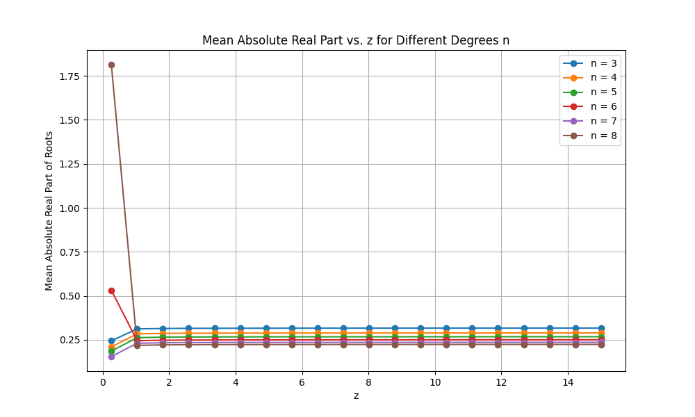
Also we found that the mean absolute real parts of all the roots in a fixed degree exhibit a kind of conjugation, as shown in Figure 8.

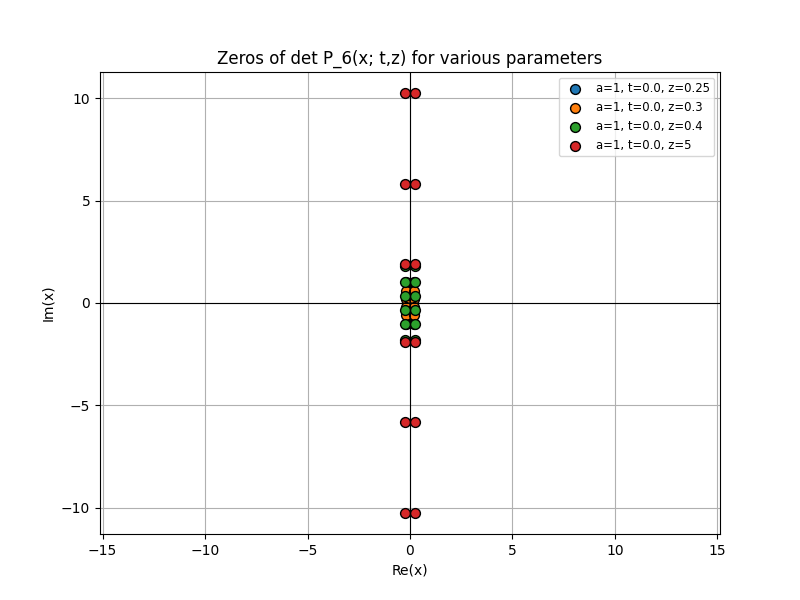
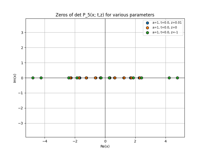
Also we can have a guess that if z is small enough then we have all real roots. Figure 9 is an example for  $$ {\text{P}}_{\text{5}}$$ 

7. Conclusion

This study aimed to investigate how Hermite polynomials—both scalar and matrix‑valued—deform under the heat‑flow partial differential equation  $$ {\text{∂}}_{\text{t}}\text{ P= }{\text{∂}}_{\text{zz}}\text{P}$$ , and the findings indicate that this evolution admits closed‑form descriptions connecting PDE dynamics, explicit formulas, and zero trajectories. The analysis revealed: (i) a Taylor‑series solution  $$ \text{P(}\text{t,z}\text{)=}\sum _{\mathrm{j}\ge 0}\frac{{\mathrm{t}}^{\mathrm{j}}}{\mathrm{j}!}{\partial }_{\mathrm{z}\mathrm{z}}^{\mathrm{j}}\mathrm{P}\left(\mathrm{z}\right)$$ ; (ii) an ODE for the zeros  $$ {\dot{\mathrm{z}}}_{\mathrm{m}}=-\sum _{\mathrm{i}\ne \mathrm{m}}\frac{2}{{\mathrm{z}}_{\mathrm{m}}-{\mathrm{z}}_{\mathrm{i}}}$$ , which explains short‑range repulsion and collective motion; and (iii) a scaling law for Hermite polynomials,  $$ {\mathrm{H}}_{\mathrm{n}}(\mathrm{z},\mathrm{t})={\mathrm{H}}_{\mathrm{n}}\left(\frac{\mathrm{z}}{\sqrt{1-4\mathrm{t}}}\right)(1-4\mathrm{t}{)}^{\mathrm{n}/2}$$ , which supports the initial hypothesis that the heat flow organizes the deformation through a simple argument rescaling together with a degree‑dependent amplitude. We further identified a reality threshold  $$ \mathrm{t}<\frac{1}{4}$$  for the zeros and outlined explicit even‑degree coefficient behavior; in the matrix‑valued setting, we observed structured conjugation patterns in deformed spectra.

This research contributes to the existing body of knowledge by unifying the PDE‑based deformation view with classical Hermite representations (including hypergeometric forms) and by giving a transparent, analytic derivation of the deformation formula that treats even/odd degrees in a single framework. The findings extend previous theories by providing evidence that the pairwise  $$ 1/({\mathrm{z}}_{\mathrm{m}}-{\mathrm{z}}_{\mathrm{i}})$$  interaction law offers a coherent mechanism for collision, complexification, and the sharp reality barrier at  $$ \mathrm{t}=\frac{1}{4}$$ , and by showing that the same heat‑flow principle can organize certain matrix‑valued orthogonal systems constructed from Hermite blocks.

This study has practical significance for spectral methods and numerical analysis. The closed-form scaling  $$ \mathrm{z}\mapsto \mathrm{z}/\sqrt{1-4\mathrm{t}}$$  and the factor  $$ (1-4\mathrm{t}{)}^{\mathrm{n}/2}$$  yields a stable parametrization of heat‑regularized Hermite bases, informs the choice of t to preserve real quadrature nodes, and supports continuation algorithms that track zeros as  $$ \mathrm{t}$$  varies. In matrix problems, the observed conjugation structure suggests computational strategies for locating determinant zeros and designing weights that maintain spectral symmetry.

This study is limited by its focus on the Hermite family and by analyzing one representative matrix weight; the matrix‑zero conjugation behavior is empirical here and not proved in full generality. One potential limitation is the assumption of simple zeros and reliance on local ODE analysis near the  $$ \mathrm{t}=\frac{1}{4}$$  threshold, which may affect the generalizability to other orthogonal families or to weights with different analytic properties.

Future study could focus on extending the analytic deformation law and zero dynamics to Laguerre, Jacobi/Chebyshev, and other classical families; establishing rigorous proofs of the matrix conjugation phenomenon; and deriving large‑n asymptotics for zero distributions under the  $$ (1-4\mathrm{t})$$  scaling. In the future, the author will also pursue structure‑preserving numerical schemes for zero evolution, stability analysis beyond first collisions, and operator‑theoretic approaches (via generating‑function PDEs and factorizations) to obtain uniform estimates near  $$ \mathrm{t}=\frac{1}{4}$$ .

Overall, this study provides new insights into how heat flow interweaves with orthogonal polynomial structure—linking PDE evolution, explicit formulas, and zero dynamics—and highlights the importance of deformation‑invariant descriptions (scaling and interaction laws) as a unifying lens for both scalar and matrix‑valued settings. By shedding light on the interplay between diffusion, algebraic structure, and spectral geometry, this research paves the way for broader applications in approximation theory and computational mathematics.

References

[1]. Tao, T. (2017, October 17). Heat flow and zeroes of polynomials. What's New. https: //terrytao.wordpress.com/2017/10/17/heat-flow-and-zeroes-of-polynomials/
[2]. Tang, T. (1993). The Hermite spectral method for Gaussian-type functions.SIAM Journal on Scientific Computing, 14(3), 594–606.
[3]. Berg, C. (2008). The matrix moment problem. In A. J. P. L. Branquinho & A. P. Foulquié Moreno (Eds.), Coimbra lecture notes on orthogonal polynomials (pp. 1–58). Nova Science Publishers.
[4]. Damanik, D., Pushnitski, A., & Simon, B. (2008). The analytic theory of matrix orthogonal polynomials.Surveys in Approximation Theory, 4, 1–85.
[5]. Hahn, W. (1935). Über die Jacobischen Polynome und zwei verwandte Polynomklassen.Mathematische Zeitschrift, 39(1), 634–638. https: //doi.org/10.1007/BF01201380
Cite this article
Liu,J. (2025). An analytic way to prove the explicit formula for Hermite polynomial after heat flow deformation and observation in 3D dimensions. Advances in Operation Research and Production Management,4(3),35-52.
Data availability
The datasets used and/or analyzed during the current study will be available from the authors upon reasonable request.
Disclaimer/Publisher's Note
The statements, opinions and data contained in all publications are solely those of the individual author(s) and contributor(s) and not of EWA Publishing and/or the editor(s). EWA Publishing and/or the editor(s) disclaim responsibility for any injury to people or property resulting from any ideas, methods, instructions or products referred to in the content.
About volume
Journal:Advances in Operation Research and Production Management
Volume number: Vol.4
Issue number: Issue 3
ISSN:3029-0880(Print) / 3029-0899(Online)
© 2024 by the author(s). Licensee EWA Publishing, Oxford, UK. This article is an open access article distributed under the terms and conditions of the Creative Commons Attribution (CC BY) license. Authors who publish this series agree to the following terms:
1. Authors retain copyright and grant the series right of first publication with the work simultaneously licensed under a Creative Commons Attribution License that allows others to share the work with an acknowledgment of the work's authorship and initial publication in this series.
2. Authors are able to enter into separate, additional contractual arrangements for the non-exclusive distribution of the series's published version of the work (e.g., post it to an institutional repository or publish it in a book), with an acknowledgment of its initial publication in this series.
3. Authors are permitted and encouraged to post their work online (e.g., in institutional repositories or on their website) prior to and during the submission process, as it can lead to productive exchanges, as well as earlier and greater citation of published work (See Open access policy for details).