1 Introduction

1.1 Background

Chicago, known for its high crime rates, faces significant quality-of-life challenges due to crime, which impacts security, fosters poverty, and contributes to educational inequality. Crime and urban economy are deeply intertwined, with factors like economic disparity, limited social services, and inadequate urban planning often leading disadvantaged neighborhoods toward criminal activity. Understanding shifts in crime trends has become especially important with the COVID-19 pandemic’s disruptions to social and economic conditions.

1.2 Literature Review

Quantifying the built environment is a crucial first step in examining its impact on crime patterns. While socio-economic factors are relatively straightforward to measure using statistical data, the built environment poses challenges due to a lack of standardized variables. Previous studies have assessed built environment characteristics through physical features identified via surveys, fieldwork, or environmental audits [2, 14, 15].

Jeffery (2021) emphasizes the role of Crime Prevention Through Environmental Design (CPTED), which considers factors like urban functions, street networks, and green spaces. Certain features, such as dense commercial venues (e.g., hotels, retail stores) and high-access public transportation areas, are linked to increased crime rates, underscoring urban functionality’s role in crime prediction [15, 12].

Mixed findings on the built environment's influence on crime suggest limitations of traditional linear models [8, 18]. Recent studies advocate for non-linear models in environmental criminology to capture these complex relationships [7, 12]. While prior studies often focused on small areas due to data constraints, some broader analyses at the city level incorporate demographic and policy dimensions but may miss the nuances of specific urban characteristics [17]. This study, therefore, explores the non-linear dynamics between built environment and socio-economic factors in influencing crime, affirming their interlinked effects.

1.3 Hypotheses and Objectives

This study examines the impact of the COVID-19 pandemic on crime trends in Chicago, focusing on three main hypotheses:

Pandemic Impact on Crime: The study hypothesizes that COVID-19 has significantly affected crime density, leading to notable shifts in crime rates during and after the pandemic.

Determinants of Crime: The built environment and socioeconomic factors are expected to play key roles in influencing crime density, with these influences varying across different phases of the pandemic.

Crime Prediction: Using crime data combined with built environment and socioeconomic determinants, the study aims to develop a predictive model to forecast crime trends in Chicago, serving as a practical tool for urban planning and crime prevention.

The study’s primary objective is to analyze and predict Chicago’s crime trends, especially regarding pandemic impacts. By examining shifts across different pandemic stages, the study seeks to identify patterns and determinants of crime, including socioeconomic and environmental factors, and understand how their influence fluctuates. An essential goal is to construct an accurate predictive model that can aid urban planning, public safety strategies, and decision-making in crime prevention. Additionally, this study contributes to existing literature by providing insights into the complex interplay between pandemics, urban environments, and crime rates, enhancing understanding of these relationships in an urban context.

1.4 Conceptual Framework

Criminal activity arises from the interaction between individuals motivated to commit a crime and the opportunity provided by a specific environment. Crime causation can be viewed from three perspectives: the motives and attitudes of offenders, the vulnerability of potential victims, and the role of the built environment and social conditions. This study focuses on the third perspective, analyzing how social and environmental characteristics influence crime density in Chicago.

As shown in Figure 1, we measure Chicago’s built environment through variables like roads, restaurants, transportation, financial institutions, and recreational spaces, while the social environment includes indicators of social disadvantage, property, and household characteristics. Research shows that built environment features directly correlate with crime; for instance, mixed land use may attract outsiders, weakening social control. Studies also suggest that vibrant areas with many grocery stores and restaurants may increase neighborhood theft, while multifamily residential and commercial zones often experience lower burglary rates than single-use properties.

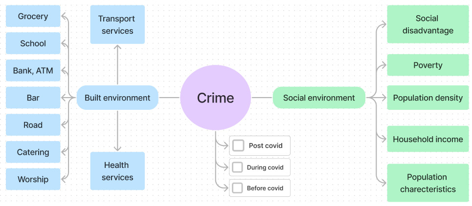
Figure 1. Research framework

2 Methodology

2.1 Date and Sources

In this study, crime-related factors are categorized into two primary groups based on literature review:

Built Environment Factors: Elements of the built environment can significantly impact crime rates. Features like poor lighting, abandoned buildings, limited green spaces, and high traffic are associated with increased crime, while well-maintained spaces with adequate lighting and strong community presence often experience lower crime rates. Urban layout also plays a role: curved streets discourage through traffic and enhance resident monitoring, generally reducing crime, while grid-like streets can facilitate escape routes and may increase crime incidents.

Specific amenities, such as schools, banks, and grocery stores, also influence crime rates in complex ways. Areas with a higher concentration of banks often report lower crime, likely due to increased economic stability and employment. Grocery stores can also contribute positively by improving access to food and quality of life, indirectly reducing crime. Green spaces have mixed effects; while dense tree cover can conceal crime, green areas often foster social interaction and deter crime through community presence. Visible security measures, such as street cameras, also contribute to reduced crime locally.

Socioeconomic Factors: Socioeconomic conditions strongly correlate with crime. Factors like poverty, unemployment, low education, and income inequality are commonly associated with higher crime rates. Poverty and unemployment are linked to crime through resource scarcity, stress, and instability. Education also plays a role, as lower educational attainment correlates with higher crime risk, often due to limited job opportunities. Income inequality, by weakening social cohesion and increasing perceived injustice, is also a significant predictor of crime rates.

These environmental and socioeconomic factors provide a comprehensive framework for analyzing the interplay between surroundings, social conditions, and crime, offering insight into broader social and environmental influences on criminal behavior.

2.2 Study Methodology

2.2.1 Traditional Regression

This study applies three linear regression models—Ordinary Least Squares (OLS), Lasso, and Ridge—to examine the relationship between independent variables and crime rates, helping to identify factors linked to higher crime rates and predict levels across different areas.

• Ordinary Least Squares (OLS): A straightforward linear model that minimizes the sum of squared errors between predicted and actual values, although it relies on assumptions about error distribution and multicollinearity.

• Lasso and Ridge Regression: These models use regularization to address OLS limitations. Lasso (L1 regularization) selects essential features by setting some coefficients to zero, reducing overfitting, while Ridge (L2 regularization) shrinks coefficient magnitudes to handle multicollinearity.

2.2.2 Machine Learning Models

Machine learning algorithms offer several advantages over traditional methods for crime analysis and prediction:

• Handling Large, Complex Data: Machine learning models are designed for analyzing extensive datasets common in crime analysis.

• Capturing Nonlinear Relationships: These models effectively capture nonlinear patterns often found in crime data, which linear regression models may miss.

• Automatic Feature Selection and Ensembling: Machine learning algorithms can identify key predictors and use ensembling techniques, like Random Forests and Gradient Boosting, to improve accuracy.

• Flexibility with Data Types: Machine learning models adapt well to various data types, including spatial and temporal data.

This study uses five machine learning models: Random Forest, Extra Trees, Gradient Boosting, K-Nearest Neighbors, and Multi-Layer Perceptron Neural Network. Performance is evaluated using six metrics: RMSE, %RMSE, MAE, %MAE, precision (P), and R-squared.

3 Descriptive Analysis

3.1 Shifting Trend of All Crime Types

This section examines the shifting trends of various crime types in Chicago across three temporal phases of the pandemic: pre-pandemic, amid-pandemic, and post-pandemic. First, it assesses temporal changes in overall crime trends, identifying patterns and pinpointing significant events that may have influenced these changes. Special attention is given to the most frequently reported crime in Chicago—namely, theft—to analyze both temporal and spatial shifts from 2020 to 2022. This analysis aims to provide a thorough understanding of Chicago's evolving crime landscape and the potential impacts of COVID-19 and its associated containment measures on crime rates in the city.

Figure 2 displays the rolling daily total of all reported crimes in Chicago from 2020 to 2022, highlighting a notable surge on May 25, 2020. This exponential increase in crime followed the death of George Floyd, an African American man who died during an encounter with police. His death triggered widespread protests, civil unrest, and a resurgence of the Black Lives Matter movement not only in Chicago but also across the United States and internationally.

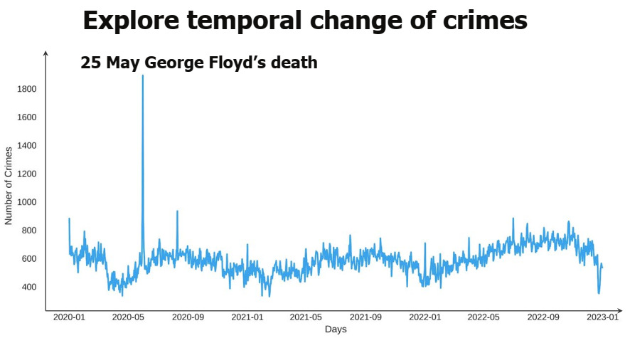
Figure 2. Rolling sum of all crimes in Chicago (2020-2022)

(Source: self-drawn)

Monthly aggregation of crime data reveals a fluctuating trend throughout the year, with crime rates typically rising during the summer months (Figure 3). This seasonal pattern may be attributed to heightened social activity and outdoor gatherings during warmer months compared to the colder winter period. Additionally, an overall increase in crime rates is observed in the post-pandemic period of 2022, which could be linked to factors such as economic hardship or the relaxation of pandemic containment measures.

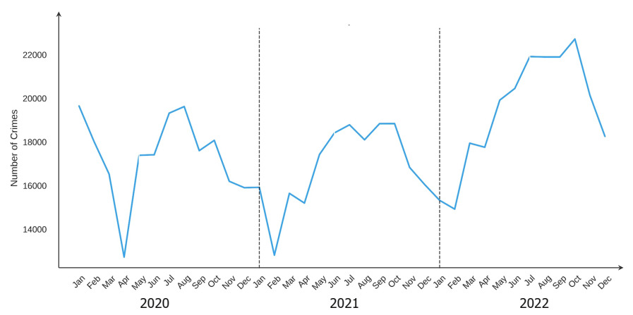
Figure 3. Number of all crimes in Chicago by month and year (2020-2022)

(Source: self-drawn)

The analysis indicates distinct trends across different crime categories during the pandemic. White-collar and drug-related crimes have consistently declined, while public order crimes initially decreased and then rose. Weapon offenses showed fluctuations, and violent crimes demonstrated a steady increase, particularly since the onset of the pandemic. Notably, property crimes saw a sharp increase following the COVID-19 outbreak, continuing on an upward trajectory.

To analyze these diverse crime types effectively, crimes were grouped into seven primary categories: violent, drug-related, weapon offenses, white-collar, public order, property crimes, and others (Table 1). Temporal trends for these categories were visualized (Figure 4). The analysis revealed a consistent decline in white-collar and drug crimes during the pandemic, contrasting with a gradual increase in public order crimes following an initial dip and fluctuations in weapon offenses. Violent crimes displayed a steady rise throughout the pandemic period, with the most pronounced increases occurring early in the outbreak. This trend may be partially attributed to pandemic-induced financial instability, which likely contributed to an increase in property crimes.

Table 1. Major categories of crime

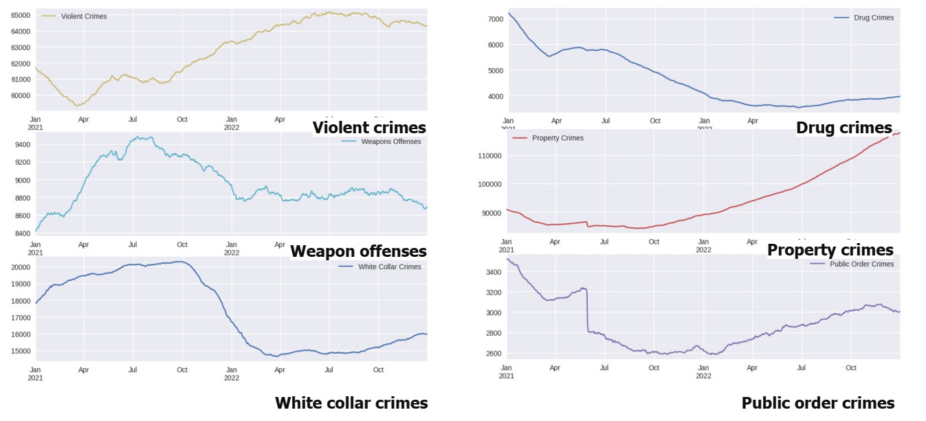
Figure 4. Temporal trend by six major crime categories in Chicago (2020-2022)

(Source: self-drawn)

Figure 5 illustrate the total number of crimes by each subtype of crimes and the shifting temporal trend by different crime types in Chicago. We observed that theft had the highest number of crimes, followed by battery, criminal damage, and assault. Furthermore, theft crimes exhibited an accelerating trend, highlighting the necessity for further analysis and exploration of the underlying causes behind theft crime changes.

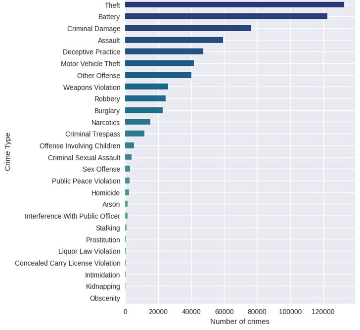
Figure 5. Total number of different sub-crime types in Chicago from 2020 to 2022

(Source: self-drawn)

3.2 Shifting Trend of Theft Crime

The shifting trend of theft crimes from 2020 to 2022 (Figure 6) reveals a decreasing pattern in the pre-pandemic period. However, following the easing of restrictions in July 2021, theft crimes began an overall upward trend, returning to pre-pandemic levels. Chicago’s phased reopening plan, "Protecting Chicago," initiated in May 2020, likely influenced these shifts in theft crime numbers, as the plan imposed varying restrictions on businesses, capacity, social distancing, and safety protocols across different phases.

The lowest point in theft crimes, observed in February 2021, may be attributed to several factors. These include strict limitations on business operations and public gatherings, which reduced potential theft targets. Additionally, February is one of Chicago’s coldest months, which may have further deterred outdoor activities, limiting opportunities for theft.

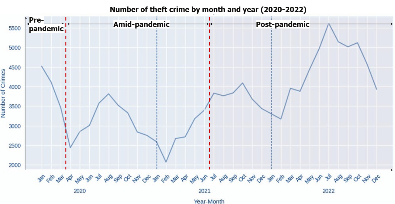
Figure 6. Change in number of theft crime in Chicago by month and year (2020-2022)

(Source: self-drawn)

A spatial analysis of theft crime distribution in Chicago was conducted, offering an overview of its spatial patterns before, during, and after the COVID-19 pandemic (Figure 7). The analysis reveals that while the city center remains the primary hotspot for theft crimes, the distribution has gradually dispersed over time, with new hotspots emerging in other areas of the city. This shift suggests a broadening spatial impact of theft crime beyond the central urban core.

4 Prediction Models

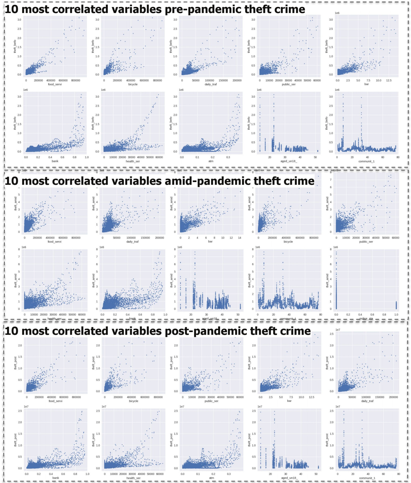
Figure 7. Distribution of test errors

To identify key variables influencing theft crime across different pandemic phases, we conducted a correlation analysis. Results showed that certain built environment features, such as food services, bicycle facilities, daily traffic, public services, bars, banks, health services, and ATMs, consistently correlated with theft crime throughout the pandemic. Additionally, socioeconomic factors, including unemployment rates and specific community areas, showed strong correlations in both pre- and post-pandemic phases. During the pandemic, variables such as bar density and proximity to police stations within a 1000m radius became more strongly correlated with theft crimes, reflecting shifts in influencing factors across different phases.

4.1 Linear Models

To assess the linear relationship between built environment, socioeconomic variables, and theft crime, we used Ordinary Least Squares (OLS) to analyze theft crime density across three phases: pre-pandemic, amid-pandemic, and post-pandemic. The baseline models yielded R² values of 0.599, 0.576, and 0.526, indicating that built environment and socioeconomic factors moderately explain variations in theft crime.

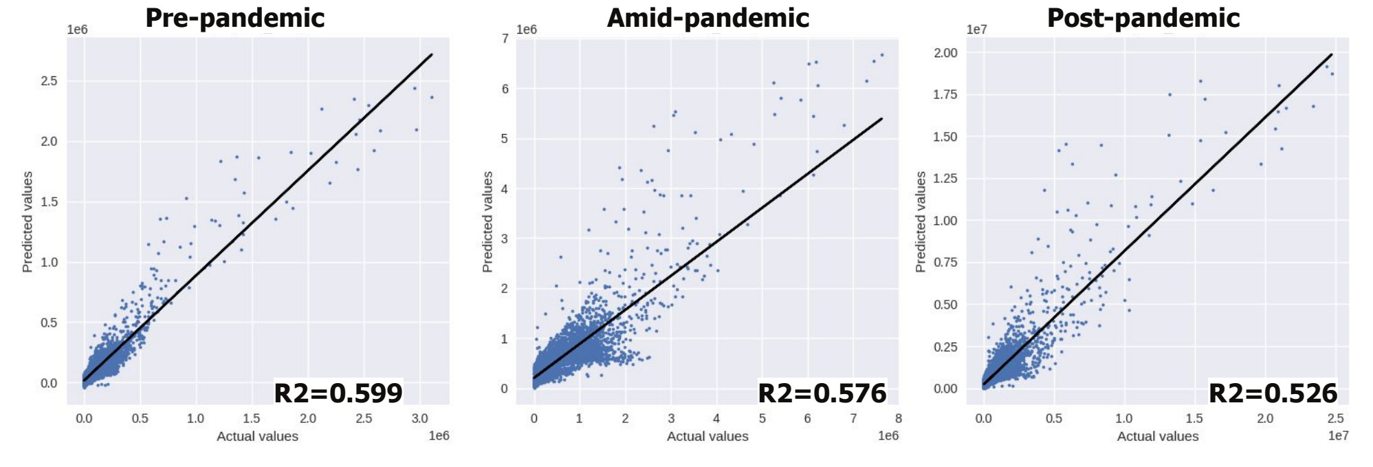
Figure 8. OLS baseline models for pre-, amid- and post-pandemic theft crimes

(Source: self-drawn)

To evaluate predictive accuracy, we split the data into 80% training and 20% testing sets and applied OLS, Lasso, and Ridge regression models with five-fold cross-validation to predict theft crime density across the pre-, amid-, and post-pandemic periods. Results indicated that OLS performed comparably to Lasso and Ridge, suggesting that regularization had minimal impact on model performance.

Table 2.OLS, Lasso and Ridge results

4.2 Non-linear exploration

After analyzing linearity with OLS, Lasso, and Ridge models, we applied machine learning models to explore non-linear relationships between built environment, socio-economic variables, and theft crime density. We used Random Forest, Extra Trees, Gradient Boosting, MLP-NN, and K-NN models. The Extra Trees model, which builds an ensemble of decision trees with randomly selected splits, emerged as the most suitable model for predicting post-pandemic theft crime in Chicago, given its lower RMSE and MAE and higher R² score (Table 2 and Figure 9). The normal distribution of test errors for the Extra Trees model further supports its reliability and accuracy (Figure 10).

Table 3. Random Forest, Extra Trees, Gradient Boosting, MLP-NN, K-NN results

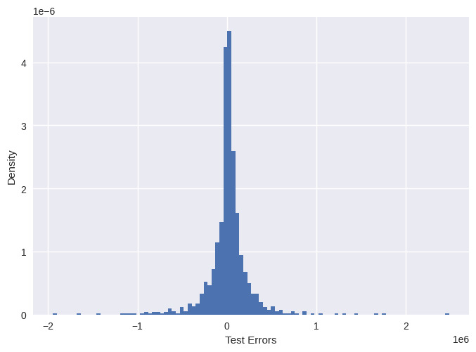
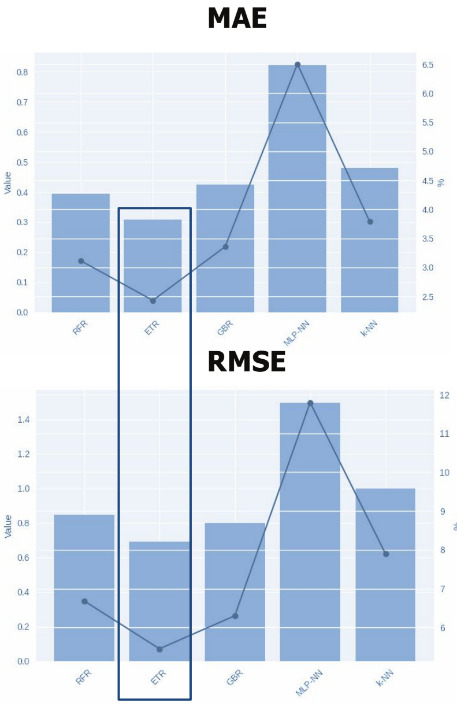
Figure 9. MAE and RMSE for machine learning models Figure 10. Distribution of test errors

This study highlights the strong influence of built environment features, such as school, grocery, and library density, road density, daily traffic volume, and density of banks, bicycle parking, and food services, on theft crime (Figure 11). These environmental features showed a stronger impact on theft crime density compared to socio-economic factors, aligning with the findings from our linear models. These results underscore the importance for urban planners and policymakers to consider built environment features in developing crime prevention strategies.

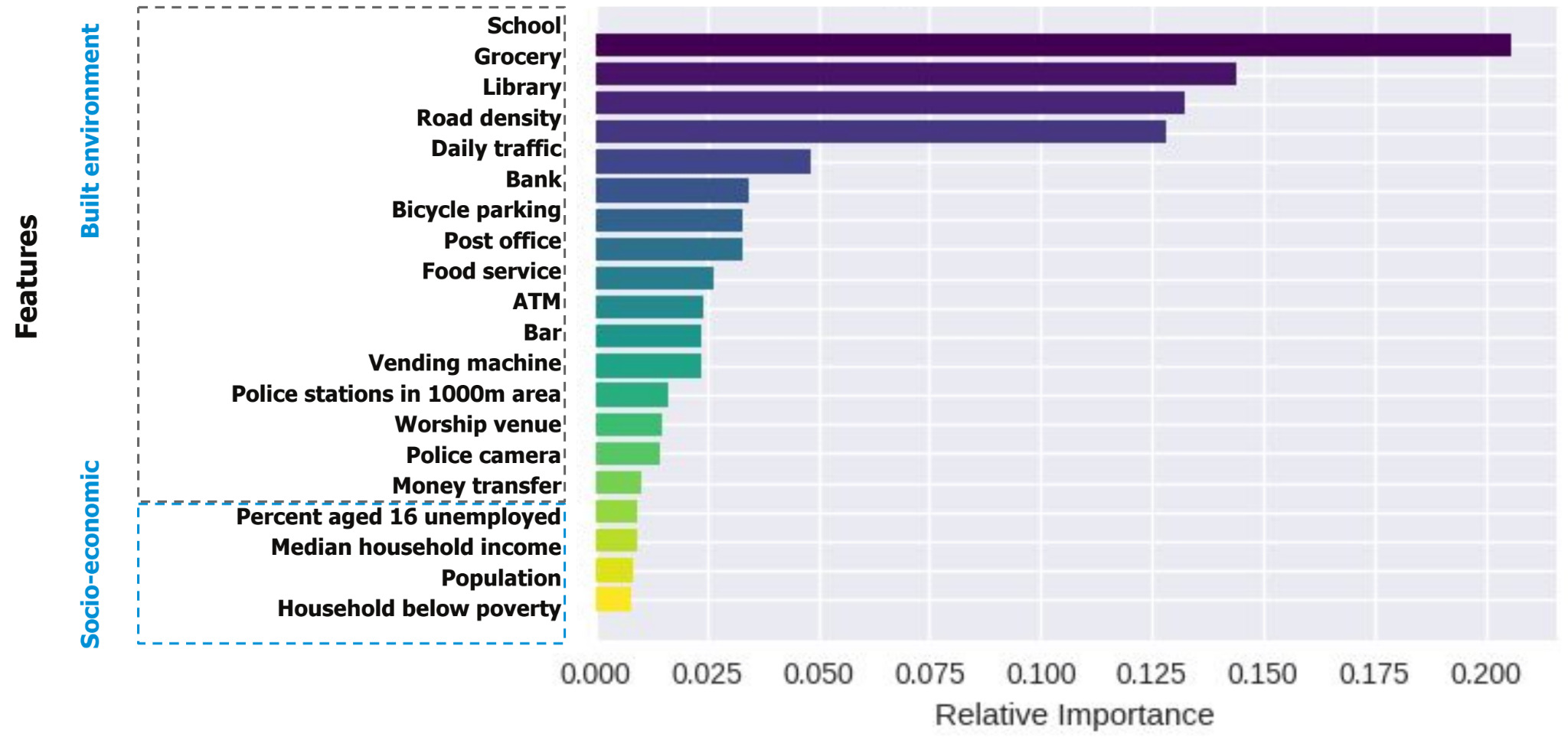
Figure 11. Feature importance of top 20 variables

(Source: self-drawn)

To further investigate, we used Partial Dependence Plots (PDPs) to analyze the threshold effects of specific features on theft crime density while considering average effects across other features. PDPs provided insights into complex relationships, showing that major environmental factors, including school, grocery, and library density, along with daily traffic, collectively contribute to higher theft crime density. The effects of socio-economic factors, however, were more nuanced. For instance, the PDP for median household income and percentage of households below the poverty line revealed threshold effects, where crime density initially rises with population increases but eventually levels off. This suggests a need for nuanced analysis of socio-economic factors in relation to crime trends.

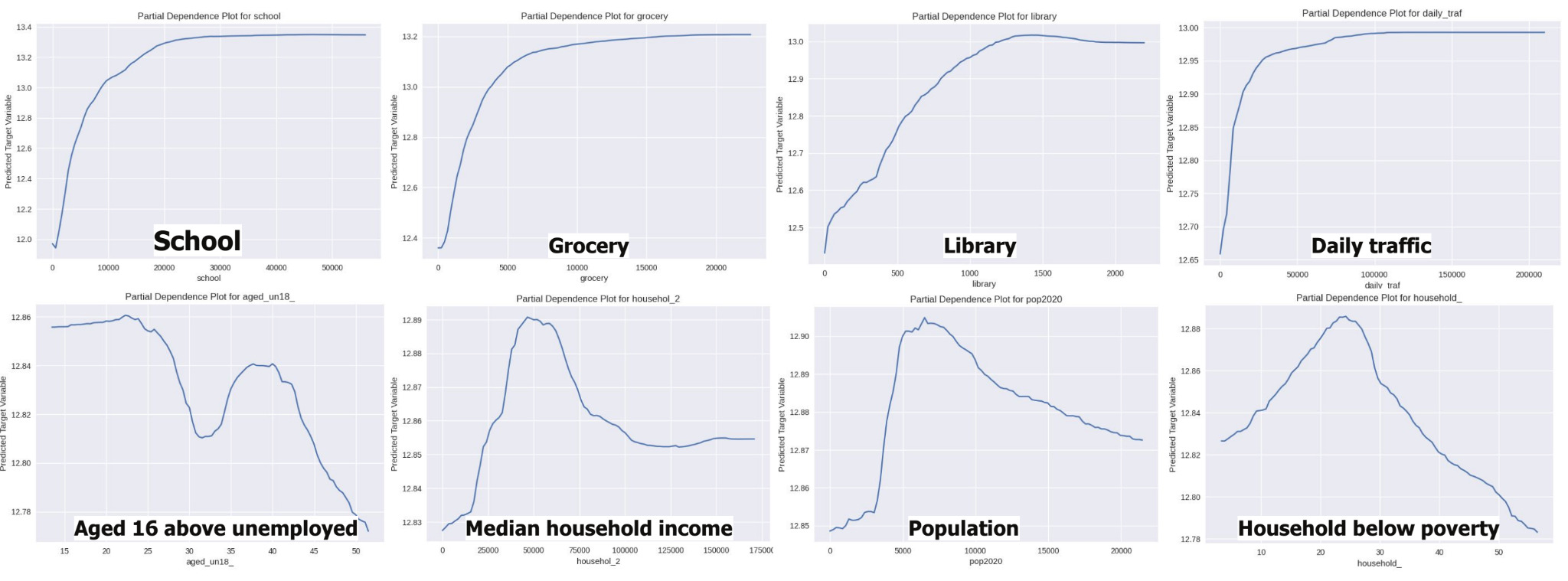
Figure 12. Partial Dependence Plots of representative built environment and socioeconomic features

(Source: self-drawn)

In summary, our comparison of linear and non-linear models indicates that non-linear machine learning models, with an R² score of 0.943, outperform linear models in capturing complex relationships influencing crime. This aligns with previous studies highlighting non-linear dynamics in factors affecting crime density.

5 Conclusions

Using a 500m fishnet grid and machine learning techniques, this study identified key variables affecting theft density in Chicago, with the Extra Trees (ETR) model outperforming others. This research findings highlight the significant role of built environment variables in influencing theft density, aligning with previous studies [4-6]. Results indicate that built environment features have a significant impact on theft density, while socio-economic factors like unemployment and income inequality show variable effects across pandemic periods. These findings suggest that urban and social factors interact to influence crime patterns, with non-linear models capturing these complex relationships more effectively than traditional methods. For policymakers and urban planners, the results underscore the importance of incorporating built environment considerations into crime prevention strategies, particularly in adapting urban spaces to foster safer, more resilient communities in the post-pandemic era.

References

[1]. Caves, R. W. (Ed.). (2005). Encyclopedia of the city (p. 676). Taylor & Francis. ISBN 978-0415862875.
[2]. Evenson, K. R., Block, R., Roux, A. V. D., McGinn, A. P., Wen, F., & Rodríguez, D. A. (2012). Associations of adult physical activity with perceived safety and police-recorded crime: The Multi-Ethnic Study of Atherosclerosis. International Journal of Behavioral Nutrition and Physical Activity, 9, 1-12.
[3]. He, L., Páez, A., Jiao, J., An, P., Lu, C., Mao, W., & Long, D. (2020). Ambient population and larceny-theft: A spatial analysis using mobile phone data. ISPRS International Journal of Geo-Information, 9(6), 342.
[4]. He, L., Páez, A., & Liu, D. (2017). Built environment and violent crime: An environmental audit approach using Google Street View. Computers, Environment and Urban Systems, 66, 83-95. https://doi.org/10.1016/j.compenvurbsys.2017.08.001
[5]. He, Q., & Li, J. (2022). The roles of built environment and social disadvantage on the geography of property crime. Cities, 121, 103471. https://doi.org/10.1016/j.cities.2021.103471
[6]. He, Z., Wang, Z., Xie, Z., Wu, L., & Chen, Z. (2022). Multiscale analysis of the influence of street built environment on crime occurrence using street-view images. Computers, Environment and Urban Systems, 97, 101865. https://doi.org/10.1016/j.compenvurbsys.2022.101865
[7]. Hipp, J. R., Lee, S., Ki, D., & Kim, J. H. (2021). Measuring the built environment with Google Street View and machine learning: Consequences for crime on street segments. Journal of Quantitative Criminology, 1-29.
[8]. Hipp, J. R., & Yates, D. K. (2011). Ghettos, thresholds, and crime: Does concentrated poverty really have an accelerating increasing effect on crime? Criminology, 49(4), 955-990.
[9]. Jeffery, C. R. (2021). Crime prevention through environmental design. Beverly Hills: Sage.
[10]. Kim, Y.-A., & Hipp, J. R. (2017). Physical boundaries and city boundaries: Consequences for crime patterns on street segments? Crime & Delinquency, 64(2), 227-254. https://doi.org/10.1177/0011128716687756
[11]. Lee, D. W., & Lee, D. S. (2020). Analysis of influential factors of violent crimes and building a spatial cluster in South Korea. Applied Spatial Analysis and Policy, 13, 759-776.
[12]. Lee, N., & Contreras, C. (2021). Neighborhood walkability and crime: Does the relationship vary by crime type? Environment and Behavior, 53(7), 753-786.
[13]. Lin, J., Wang, Q., & Huang, B. (2021). Street trees and crime: What characteristics of trees and streetscapes matter? Urban Forestry & Urban Greening, 65, 127366.
[14]. Loukaitou-Sideris, A., Liggett, R., Iseki, H., & Thurlow, W. (2001). Measuring the effects of built environment on bus stop crime. Environment and Planning B: Planning and Design, 28(2), 255-280.
[15]. Moniruzzaman, M., & Páez, A. (2012). A model-based approach to select case sites for walkability audits. Health & Place, 18(6), 1323-1334.
[16]. Summers, L., & Johnson, S. D. (2017). Does the configuration of the street network influence where outdoor serious violence takes place? Using space syntax to test crime pattern theory. Journal of Quantitative Criminology, 33, 397-420.
[17]. Vélez, M. B., Lyons, C. J., & Santoro, W. A. (2015). The political context of the percent black-neighborhood violence link: A multilevel analysis. Social Problems, 62(1), 93-119.
[18]. Wheeler, A. P., & Steenbeek, W. (2021). Mapping the risk terrain for crime using machine learning. Journal of Quantitative Criminology, 37, 445-480.
Cite this article
Wang,X. (2024). Exploring the Impact of Socioeconomic and Built Environment Factors on Theft Crime Trends in Chicago During the COVID-19 Pandemic. Journal of Applied Economics and Policy Studies,14,21-30.
Data availability
The datasets used and/or analyzed during the current study will be available from the authors upon reasonable request.
Disclaimer/Publisher's Note
The statements, opinions and data contained in all publications are solely those of the individual author(s) and contributor(s) and not of EWA Publishing and/or the editor(s). EWA Publishing and/or the editor(s) disclaim responsibility for any injury to people or property resulting from any ideas, methods, instructions or products referred to in the content.
About volume
Journal:Journal of Applied Economics and Policy Studies
© 2024 by the author(s). Licensee EWA Publishing, Oxford, UK. This article is an open access article distributed under the terms and
conditions of the Creative Commons Attribution (CC BY) license. Authors who
publish this series agree to the following terms:
1. Authors retain copyright and grant the series right of first publication with the work simultaneously licensed under a Creative Commons
Attribution License that allows others to share the work with an acknowledgment of the work's authorship and initial publication in this
series.
2. Authors are able to enter into separate, additional contractual arrangements for the non-exclusive distribution of the series's published
version of the work (e.g., post it to an institutional repository or publish it in a book), with an acknowledgment of its initial
publication in this series.
3. Authors are permitted and encouraged to post their work online (e.g., in institutional repositories or on their website) prior to and
during the submission process, as it can lead to productive exchanges, as well as earlier and greater citation of published work (See
Open access policy for details).