1. Introduction

Quantitative trading primarily employs mathematical models, statistical methods, and computer algorithms to analyze market data, formulating, executing, and managing trading decisions. This approach systematically and automatically executes trades, minimizing human intervention, and often covers multiple financial instruments and markets. The advantage of quantitative trading lies in its elimination of emotional biases, turning investment strategies into systematic rules, and striving for stable returns through data and models.

Due to its strong performance in fund allocation management, the Kelly formula has found widespread use in fields such as statistical arbitrage and trend-following quantitative trading. The Kelly formula helps quantitative investors manage positions and control risk by adjusting investment proportions according to market conditions, thus maximizing long-term investment returns. However, since the Kelly formula assumes that traders can accurately estimate win probabilities and returns, which is often difficult to achieve in practice, relying entirely on the Kelly formula for fund allocation can lead to overly aggressive strategies, resulting in high return volatility and, in extreme cases, substantial short-term losses. Therefore, this paper introduces the concept of the overfitting rate to improve the Kelly formula, overcoming the issues that may arise during long-term quantitative trading investments, and optimizing quantitative trading strategies.

In the field of portfolio management, many scholars have focused on optimizing asset allocation using the Kelly formula to achieve the maximum growth of wealth. Markowitz, in his Modern Portfolio Theory, first proposed using portfolio variance as a measure of risk, emphasizing the importance of risk control in investment [1]. In 1956, American scholar J. Kelly first introduced the Kelly formula, which provides a scientific method for selecting the optimal bet ratio in gambling and investment situations to achieve the long-term maximization of wealth [2]. When researchers applied the Kelly model to the securities investment market, Thorp and Rotando proved that under continuous distributions, the wealth growth rate has a unique maximum value [3]. MacLean, Thorp, and Ziemba conducted a comprehensive analysis of the Kelly optimization model, demonstrating that the Kelly formula not only has significant theoretical advantages but also proves capable of delivering returns that surpass traditional investment strategies in practical applications [4]. However, despite its outstanding performance in long-term investments, the high risk associated with the Kelly formula presents a significant challenge in practical use, particularly during times of severe market fluctuations. To address this, MacLean, Ziemba, and Blazenko proposed a partial Kelly strategy, where part of the Kelly score is allocated to risky investments and the rest to risk-free investments, thereby reducing risk while maintaining a solid growth rate [5]. Jacquier and Polson integrated the Kelly criterion into a unified statistical inference framework using Bayesian methods, further correcting the errors in the Kelly criterion under non-normal conditions [6]. Wu M. E., Tsai H. H., and Chung W. H. utilized Kullback-Leibler divergence to describe the relationship between actual profits, losses, and expected values, further demonstrating that the Kelly criterion can be used to obtain the optimal betting solution under a limited number of gambling trials [7]. Additionally, Carta and Conversano developed and designed a framework for applying the Kelly criterion in the stock market, using Monte Carlo simulations in different scenarios to show that the Kelly criterion maximizes the expected growth rate and median terminal wealth compared to other investment methods [8].

Based on the above research, this paper applies the Kelly criterion in continuous time to the quantitative trading market and improves the Kelly formula in response to the overfitting problem in quantitative trading. By using a sliding window method to update the Kelly score in real-time, the strategy more rationally determines the order ratio, effectively hedges risks, and achieves stable long-term expected return maximization.

2. Model Setup

2.1. Discrete Distribution

The original model of the Kelly formula is based on discrete distributions:

1. Consider an investor making multiple independent bets (such as a coin toss experiment).

2. Assume the coin is biased, with a win probability of \( p \gt \frac{1}{2} \) , and a failure probability of \( q=1-p \) .

3. The initial wealth is \( {W_{0}} \) , and for each win, the invested amount is doubled, while for each loss, the invested amount is zeroed out.

4. The objective is to determine the optimal betting fraction that maximizes long-term wealth growth.

Let \( {W_{n}} \) denote the wealth after the n-th investment, and \( {B_{k}} \) the amount invested on the k-th bet. If the k-th bet is a win, then \( {T_{k}}=1 \) , and if it is a loss, \( {T_{k}}=-1 \) . The expected value of \( {W_{n}} \) is:

\( E({W_{n}})={W_{0}}+\sum _{k=1}^{n}E({B_{k}}{T_{k}})={W_{0}}+\sum _{k=1}^{n}(p-q)E({B_{k}}) \)

Assume there is a parameter \( 0 \lt f \lt 1 \) such that the investment on the k-th bet is \( {B_{k}}=f{W_{i-1}} \) . After n bets, the wealth becomes:

\( {W_{n}}={(1+f)^{S}}∙{(1-f)^{F}} \)

Where S and F represent the number of successes and failures, respectively, with \( S+F=n \) .

Thus, the expected logarithmic growth rate of total wealth is:

\( G(f)=E\lbrace {ln{[\frac{{W_{n}}}{{W_{0}}}]}^{\frac{1}{n}}}\rbrace =E\lbrace \frac{S}{n}ln{(1+f)}+\frac{F}{n}ln{(1-f)\rbrace =pln{(1+f)}+q}ln{(1-f)} \)

Taking the derivative of \( G(f) \) :

\( {G^{ \prime }}(f)=\frac{p}{1+f}-\frac{q}{1-f}=\frac{p-q-f}{(1+f)(1-f)} \)

Taking the second derivative:

\( {G^{ \prime \prime }}(f)=\frac{-{f^{2}}+2f(p-q)-1}{{(1-{f^{2}})^{2}}} \lt 0 \)

Therefore, the logarithmic growth rate reaches its maximum when \( {f^{*}}=p-q \) . When the odds are \( b \) , the optimal Kelly score is:

\( {f^{*}}=\frac{bp-q}{b} \)

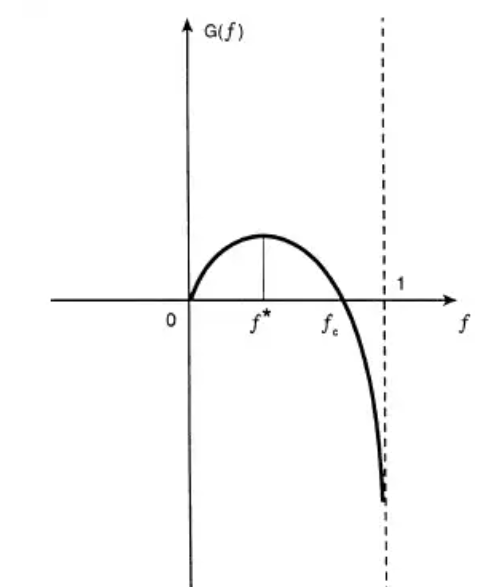
Figure 1. Relationship between logarithmic growth rate and betting fraction under discrete distribution for the Kelly formula

2.2. Continuous Distribution

In the stock market, stock prices can be approximated as continuous variables, and holding a stock is a continuous action. To apply the Kelly formula to the stock market, we need to approximate the original formula for continuous distributions.

Let X represent the random variable for unit investment return, where \( E(X)=μ \) and \( Var(X)={σ^{2}} \) . Suppose the initial capital \( {V_{0}} \) is invested in \( X \) at a fraction \( f \) , then the total capital after one investment cycle is given by:

\( V(f)={V_{0}}(1+(1-f)r+fX) \)

Where r is the risk-free return rate on the remaining capital. If we divide one investment cycle into n independent and equally-sized investments, while maintaining the overall return and variance, then after n investments, the return rate is:

\( {G_{n}}(f)=\frac{{V_{n}}(f)}{{V_{0}}}=\prod _{i=1}^{n}(1+(1-f)\frac{r}{n}+f{X_{i}}) \)

Taking the expected logarithm on both sides yields \( {g_{n}}(f) \) :

\( {g_{n}}(f)=\sum _{i=1}^{n}E[ln{(1+(1-f)\frac{r}{n}+f{X_{i}})}] \) \( =\sum _{i=1}^{n}\frac{1}{2}ln{(1+\frac{r}{n}+f(\frac{μ}{n}-\frac{r}{n}+\frac{σ}{\sqrt[]{n}}))+\frac{1}{2}ln{(1+\frac{r}{n}+f(\frac{μ}{n}-\frac{r}{n}-\frac{σ}{\sqrt[]{n}})})} \) \( =\frac{n}{2}*[ln{(1+\frac{r}{n}+f(\frac{μ}{n}-\frac{r}{n}+\frac{σ}{\sqrt[]{n}}))}+\frac{1}{2}ln{(1+\frac{r}{n}+f(\frac{μ}{n}-\frac{r}{n}-\frac{σ}{\sqrt[]{n}}))}] \)

Using a Taylor expansion:

\( ln{(1+x)}=x-\frac{{x^{2}}}{2}+\frac{{x^{3}}}{3}-… \)

To simplify the calculations, let:

\( x=\frac{r}{n}+f(\frac{μ}{n}-\frac{r}{n}+\frac{σ}{\sqrt[]{n}}) \)

and

\( y=\frac{r}{n}+f(\frac{μ}{n}-\frac{r}{n}-\frac{σ}{\sqrt[]{n}}) \)

Substituting these into the equation:

\( {g_{n}}(f)=\frac{n}{2}*[x+y-\frac{{x^{2}}}{2}-\frac{{y^{2}}}{2}+O({n^{-2}})] \)

Notice:

\( x+y=2(\frac{r}{n}+f(\frac{μ}{n}-\frac{r}{n})) \)

and

\( \frac{{x^{2}}}{2}+\frac{{y^{2}}}{2}={f^{2}}\frac{{σ^{2}}}{n}+O({n^{-\frac{2}{3}}}) \)

Substituting these into the equation:

\( {g_{n}}(f)=r+f(μ-r)-\frac{{f^{2}}{σ^{2}}}{2}+O({n^{-\frac{1}{2}}}) \)

Taking the limit as \( n→∞ \) , we get:

\( {g_{∞}}(f)=r+f(μ-r)-\frac{{f^{2}}{σ^{2}}}{2} \)

To maximize this expression, we can find the optimal investment fraction:

\( {f^{*}}=\frac{μ-r}{{σ^{2}}} \)

3. Model Optimization

Overfitting is an important and common problem in the field of machine learning. It refers to the scenario where a model performs well on the training data but struggles to maintain the same level of performance on new, unseen data. In quantitative trading, various mathematical models and computer programs are used to guide investment decisions, which inevitably leads to the issue of overfitting. Overfitting may cause investment models to become overly dependent on historical data, thus affecting the accuracy of predictions. This is particularly true in financial markets, where financial data itself is noisy, causing machine learning models to overfit the random fluctuations in historical data and fail to generalize well to future data. Therefore, the concept of overfitting rate is introduced, and it is used to adjust the optimal Kelly fraction to reduce the risk associated with model overfitting, thus balancing returns and risks.

The overfitting rate \( α(0≤α≤1) \) represents the degree of overfitting of the quantitative trading prediction model. When α=0, there is no overfitting, and when α=1, the model is fully overfitted. By using the overfitting rate α to adjust the Kelly leverage, we multiply the Kelly fraction by a conservative factor. This reduces the betting amount on the investment side to counteract potential model errors. The formula is expressed as:

\( f_{a}^{*}=(1-α)∙{f^{*}} \)

Where \( f_{a}^{*} \) represents the adjusted Kelly leverage, and α is the overfitting rate. The higher the overfitting rate, the lower the adjusted Kelly leverage, resulting in a more conservative betting fraction. Depending on the model’s degree of overfitting, the optimal Kelly leverage can be adjusted continually to effectively reduce the investment fraction and meet the goal of lowering risk while maximizing long-term returns.

In the financial field, the Information Coefficient (IC) is a commonly used indicator to measure the predictive power of a model, especially the correlation between predicted signals and actual returns. It is often used in portfolio management, risk-adjusted returns, and quantitative strategy evaluation. We can quantify the overfitting rate α using the Information Coefficient.

The IC is calculated using the following formula:

\( IC=\frac{Cov(X,Y)}{{σ_{X}}{σ_{Y}}} \)

Where:

X is the predicted return, Y is the actual return, \( Cov(X,Y) \) is the covariance between the predicted and actual returns, \( {σ_{X}} \) and \( {σ_{Y}} \) are the standard deviations of the predicted and actual returns, respectively.

Steps to calculate IC:

1. Collect time series data for predicted returns and actual returns.

2. Calculate the mean of predicted returns X and actual returns Y.

3. Calculate the covariance between X and Y.

4. Calculate the standard deviations \( {σ_{X}} \) and \( {σ_{Y}} \) .

5. Calculate the Information Coefficient.

In the context of a quantitative trading training model, let \( {IC_{train}} \) be the Information Coefficient of the training set, and \( {IC_{val}} \) be the Information Coefficient of the validation (test) set. The difference between the Information Coefficients of the training and test sets can reflect the degree of overfitting of the model. Typically, \( {IC_{train}} \gt {IC_{val}} \) , and the larger the difference, the greater the overfitting of the model.

We can quantify the overfitting rate α based on the difference between the two ICs:

\( α=\frac{{IC_{train}}-{IC_{val}}}{{IC_{train}}} \)

Therefore, we can derive the overfitting rate based on the Information Coefficient difference and apply it to adjust the optimal Kelly fraction.

The optimized optimal Kelly fraction can be expressed as:

\( f_{a}^{*}=(1-α)∙{f^{*}}=(1-\frac{{IC_{train}}-{IC_{val}}}{{IC_{train}}})∙\frac{μ-r}{{σ^{2}}}=\frac{{IC_{val}}}{{IC_{train}}}∙\frac{μ-r}{{σ^{2}}} \)

Example (based on Linear Regression Model):

1. Suppose we have a dataset for a particular stock over several days (e.g., 100 days) including features such as open price, close price, and trading volume. Using a linear regression model, we predict future stock prices based on these input features.

2. The linear regression formula is established as follows:

\( ŷ={β_{0}}+{β_{1}}{X_{1}}+{β_{2}}{X_{2}}+{β_{3}}{X_{3}}+ϵ \)

Where:

\( ŷ \) is the predicted unit investment return, \( {X_{1}} \) , \( {X_{2}} \) and \( {X_{3}} \) are the feature variables, \( {β_{0}} \) is the intercept, \( {β_{1}} \) , \( {β_{2}} \) and \( {β_{3}} \) are the regression coefficients.

3. Split the data into a training set and a test set. The first 80 days are used for training, and the remaining 20 days are used for testing. Use the regression model for prediction and testing, then calculate the initial Information Coefficient and overfitting rate based on the difference between predicted returns and actual returns.

3. Using the formula \( f_{a}^{*}=\frac{{IC_{val}}}{{IC_{train}}}∙\frac{μ-r}{{σ^{2}}} \) , calculate the initial optimal Kelly fraction, where \( μ \) is the predicted unit investment return \( ŷ \) , and \( {σ^{2}}=\frac{1}{n-k}\sum _{t=1}^{n}{({y_{t}}-{ŷ_{t}})^{2}} \) , with k being the number of features in the regression model.

4. Based on the calculated optimal Kelly fraction, invest on day 1. Collect the predicted and actual returns for day 1, add them to the dataset, remove the oldest day's data, and repeat the process of calculating the optimal Kelly fraction, investing, and updating the data as described above.

This method ensures that the training and test sets are continuously updated, maintaining the real-time accuracy of the Information Coefficient and overfitting rate. It prevents potential losses from excessive risk aversion due to fixed proportions, and allows for maximizing long-term returns while mitigating risk.

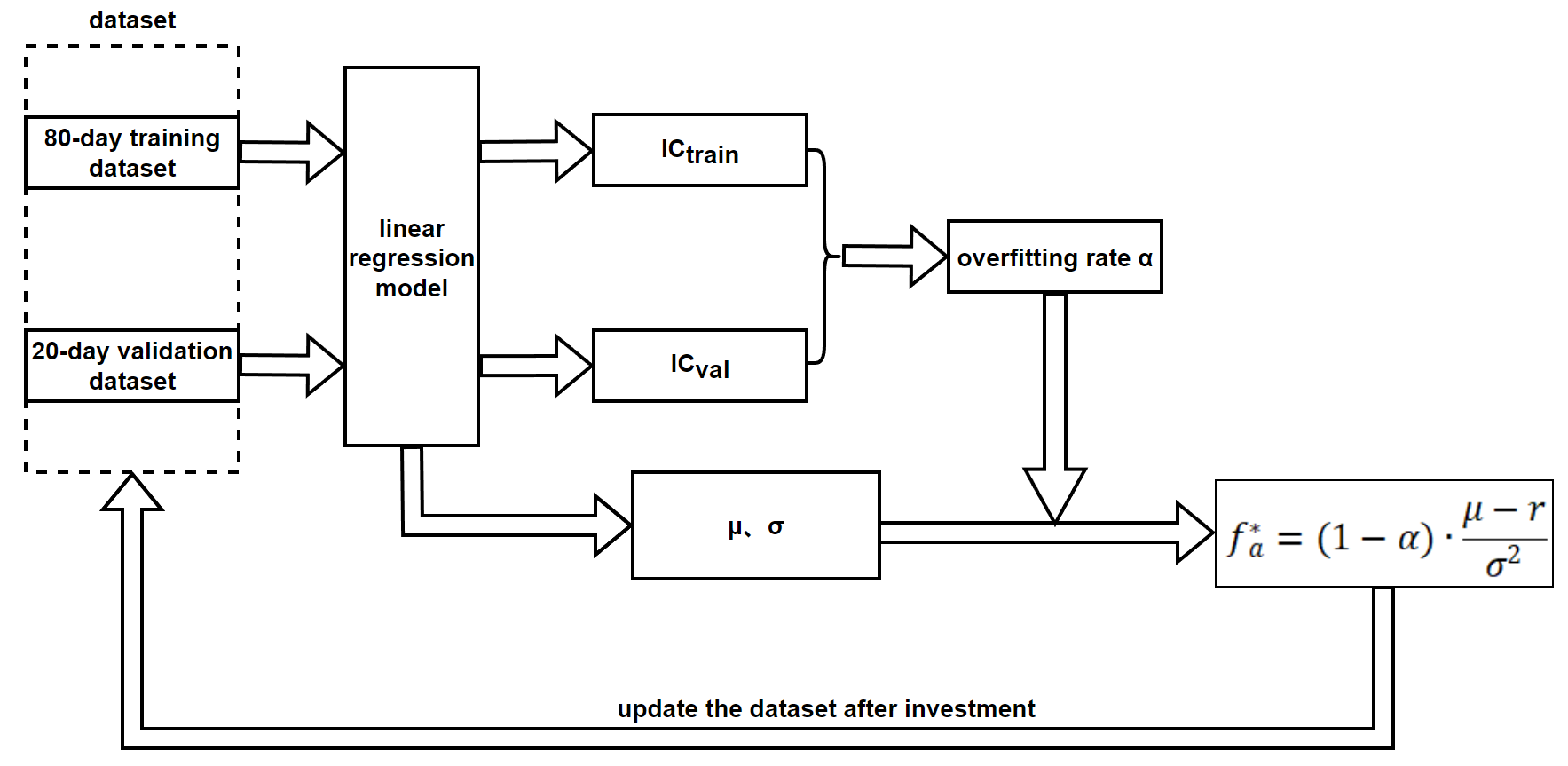
Figure 2. Model Optimization Flowchart

4. Strategy Analysis

The Kelly formula is used to calculate the optimal betting fraction or investment fraction to maximize the long-term growth rate of capital. The goal of the Kelly formula is to maximize the logarithmic growth of capital, that is, to maximize the geometric mean growth rate of the investment portfolio. Logarithmic growth has an additive property, which means that each investment seeks to use as much capital as possible to achieve long-term compounding effects. To achieve this, the Kelly formula tends to recommend a higher investment fraction, especially when both the odds and probability of success are high. This makes the Kelly formula's investment strategy inherently aggressive, potentially leading to significant volatility and investment risk.

The Fractional Kelly formula is the most commonly used risk control method based on the Kelly formula. It is a conservative variation derived from the original Kelly formula to address the volatility and investment risks associated with the original formula. The aim is to reduce investment risk, particularly when the market is highly uncertain. The Fractional Kelly formula reduces the investment fraction by multiplying the Kelly fraction by a fixed factor less than 1 (e.g., 0.5). By reducing the fixed investment fraction, the Fractional Kelly formula can help avoid investment losses due to market fluctuations. While more robust in uncertain markets, it still ignores prediction model errors and the incompleteness of market changes. In highly uncertain market environments, the Fractional Kelly formula may fail to fully capitalize on potential market opportunities, often sacrificing long-term returns.

On the other hand, introducing an overfitting rate adjustment to the Kelly formula can effectively address these shortcomings and enhance the overall risk control ability.

Table 1. Comparison of Fractional Kelly Formula and Overfitting Rate-Adjusted Kelly Formula

5. Conclusion and Recommendations

In practical investment markets, particularly in the stock market, quantitative trading models are often affected by overfitting. By incorporating the overfitting rate adjustment into the Kelly formula, we can represent the overfitting factor in quantitative trading as the overfitting coefficient α, which influences the final investment fraction with the help of the Information Coefficient. Additionally, the use of a sliding window approach in calculating the overfitting rate allows for timely updates of daily data. This ensures that the data is constantly refreshed, meeting the real-time data requirements of quantitative trading and ensuring that the trades executed each day are in alignment with the latest market conditions. As a result, this improves the adaptability and risk control capabilities of the Kelly formula in dynamic markets.

The overfitting-adjusted Kelly formula not only maintains a high expected return but also reduces the potential for loss by lowering the investment fraction. This approach not only considers risk control but also strives to maintain high investment returns, thereby achieving a more robust investment strategy. In theory, the adjusted Kelly formula offers better risk-adjusted returns in dynamic markets, which is particularly crucial for investors facing market uncertainty.

References

[1]. Markowitz, H. (1952). Portfolio selection. The Journal of Finance, 7(1), 77-91.
[2]. Kelly, J. (1956). A new interpretation of the information rate. Bell System Technical Journal, 35(4), 917-926.
[3]. Rotando, L. M., & Thorp, E. O. (1992). The Kelly criterion and the stock market. The American Mathematical Monthly, 99(10), 922-931.
[4]. Maclean, L. C., Thorp, E. O., & Ziemba, W. T. (2010). Long-term capital growth: The good and bad properties of the Kelly and fractional Kelly capital growth criteria. Quantitative Finance, 10(7), 681-687.
[5]. Davis, M. H. A., & Lleo, S. (2010). Fractional Kelly strategies for benchmarked asset management. In L. C. MacLean, E. O. Thorp, & W. T. Ziemba (Eds.), The Kelly Capital Growth Investment Criterion: Theory and Practice (pp. 127-152). World Scientific.
[6]. Jacquier, E., & Polson, N. G. (2012). Asset allocation in finance: A Bayesian perspective. In Hierarchical models and MCMC: A Tribute to Adrian Smith (pp. 56-59).
[7]. Wu, M. E., Tsai, H. H., Chung, W. H., et al. (2020). Analysis of Kelly betting on finite repeated games. Applied Mathematics and Computation, 373, 125028.
[8]. Carta, A., & Conversano, C. (2020). Practical implementation of the Kelly criterion: Optimal growth rate, number of trades, and rebalancing frequency for equity portfolios. Frontiers in Applied Mathematics and Statistics, 6, 577050.
Cite this article
Zhang,Z.;Chen,X.;Li,X. (2025). A Kelly Quantitative Trading Investment Strategy Improved by Overfitting Rate. Journal of Applied Economics and Policy Studies,17,50-55.
Data availability
The datasets used and/or analyzed during the current study will be available from the authors upon reasonable request.
Disclaimer/Publisher's Note
The statements, opinions and data contained in all publications are solely those of the individual author(s) and contributor(s) and not of EWA Publishing and/or the editor(s). EWA Publishing and/or the editor(s) disclaim responsibility for any injury to people or property resulting from any ideas, methods, instructions or products referred to in the content.
About volume
Journal:Journal of Applied Economics and Policy Studies
© 2024 by the author(s). Licensee EWA Publishing, Oxford, UK. This article is an open access article distributed under the terms and
conditions of the Creative Commons Attribution (CC BY) license. Authors who
publish this series agree to the following terms:
1. Authors retain copyright and grant the series right of first publication with the work simultaneously licensed under a Creative Commons
Attribution License that allows others to share the work with an acknowledgment of the work's authorship and initial publication in this
series.
2. Authors are able to enter into separate, additional contractual arrangements for the non-exclusive distribution of the series's published
version of the work (e.g., post it to an institutional repository or publish it in a book), with an acknowledgment of its initial
publication in this series.
3. Authors are permitted and encouraged to post their work online (e.g., in institutional repositories or on their website) prior to and
during the submission process, as it can lead to productive exchanges, as well as earlier and greater citation of published work (See
Open access policy for details).