Introduction

Generally, in the fields of electrical engineering and signal processing, the use of filters is crucial for various applications. The design purpose of a filter is to eliminate or attenuate unwanted frequencies in the signal and allow the desired frequency to pass through. The two commonly used filters are the Chebyshev filter and the Butterworth filter. In this article, the impulse response invariant method is used to design two kinds of filters, it will compare and evaluate these two types of filters, considering their frequency response, transition bandwidth, filter order, design complexity, and target application.

Chebyshev filters are divided into type I and Type II filters according to their frequency response characteristics, which fluctuate in the frequency response amplitude of the passband or stopband. These filters are known to be able to achieve sharper roll-downs in stopbands while allowing for ripples in the passband. This makes them suitable for applications that require high levels of stopband attenuation, even at the expense of passband ripple. Chebyshev filters are commonly used in radio communication systems, audio systems, and instrumentation.

The maximum flatness of the frequency response curve within the passband is a property of the Butterworth filter, with the passband unchanged and the stopband slowly decreasing to zero. As the angular frequency increases, the amplitude gradually decreases from a specific boundary angular frequency and tends to negative infinity on a log-Bode plot of amplitude and angular frequency [1]. This feature makes it suitable for applications that prioritize smooth frequency response over sharp drop characteristics. Therefore, Butterworth filters are used in audio systems, medical imaging, and telecommunications.

When choosing between Chebyshev filters and Butterworth filters, several factors need to be considered.

Firstly, In the transition band, Chebyshev filters decay with greater speed than Butterworth filters, even though whose amplitude-frequency characteristics are not as flat compared with those of the latter. The frequency response of the filter determines its performance at different frequencies. The conversion bandwidth defines the frequency range of the filter from pass to stopband. The complexity of the design may be affected by the order of the filters, i.e., the number of reactive electronic components (inductors or capacitors) necessary for the filter to operate. Finally, the target application influences the selection of the filter, as different applications may have different requirements for frequency selectivity and passband characteristics.

In this paper, it will analyze and compare the performance of Chebyshev and Butterworth filters in the case of fir filters in different scenarios, and explore in which cases and in which cases smoother frequency response is preferred. Our goal is to provide insights into the appropriate use and potential benefits of Chebyshev and Butterworth filters by studying frequency response, transition bandwidth, filter sequence, design complexity, and target applications.

Impulse response invariant design filter

The fundamental principle of the Chebyshev and Butterworth filter design is ensuring that digital filter match the analog filter’s impulse response \(h_{a}(t)\) by using unit sampling reacting sequences. Because the pulse response of the analog filter, \(h_{a}(t)\), is sampled at similar intervals, the digital filter’s unit sampling, \(h(n)\), is almost equivalent to the sampling value of the analog filter, \(h_{a}(t)\):

\(h(n) = h_{a}(t)|_{t = nt} = h_{a}(nT)\) (1)

Where T is the sampling period. The relationship between analogy frequency \(\Omega\) and digital frequency \(\omega\) is as follows:

\(\omega = \Omega T\cdots e^{j\omega} = e^{j\Omega T}\) (2)

Let \(H_{a}(s)\) represent an analog filter’s system function and \(H(z)\) represent a digital filter’s system function. It is evident that \(H_{a}(s)\) corresponds to the Laplace transform of \(h_{a}(t)\) [2]. The relationship between the Laplace transform of an analogy signal and the z-transform of its sampling sequence is:

\({H(z)|}_{z = e^{sT}} = \frac{1}{T}\sum_{k = - \infty}^{\infty}{H_{a}(j\frac{\Omega}{T} - j\frac{2\pi}{T}k)}\) (3)

It is obtained that the digital filter’s system function \(H(z)\) is obtained by the extension of the analogy filter system’s function \(H_{a}(s)\) and the mapping of \(z = e^{sT}\) to transform the analogy filter into a digital filter. Assuming that in the S-plane, the digital filter’s frequency response is determined by valuing s on the j axis and z on the unit radius \(e^{jw}\) in the Z-plane.

\(H\left( e^{jw} \right) = \frac{1}{T}\sum_{k = - \infty}^{\infty}{H_{a}(j\frac{\Omega}{T} - j\frac{2\pi}{T}k)}\) (4)

However, the frequency response of any practical analogue filter cannot be appropriately band-limited, leading to the inescapable appearance of frequency overlap, or aliasing distortion. The frequency response of a digital filter cannot be compared with that of an analog filter. Only when the comparable filter’s frequency response drastically falls after the folding frequency and the aliasing distortion is modest can the digital filter established satisfy the design requirements.

According to the principle of pulse response invariance, the process of designing the digital filter’s system function \(H(z)\) is using this method as follows: using the system function\(\ H_{a}(s)\), calculate its Laplace inverse transformation to obtain the pulse response \(h_{a}(t)\), and then perform equally spaced sampling on it:

\({h_{a}(t)|}_{t = nT} = h_{a}(nT) = h(n)\) (5)

Then calculate the z-transform of \(h(n)\) to obtain the system function \(H(z)\), which is:

\(H_{a}(s) \rightarrow h_{a}(t) \rightarrow h(n) \rightarrow H(z)\) (6)

The process described above is usually quite cumbersome, and in practice, the impulse response invariant method is particularly suitable for simulating situations where filter system functions can be represented by partial fractional expansions.

If the analog filter’s system function \(H_{a}(s)\) has just one order pole and \(M < N\), The following partial fraction representation of the system function is possible:

\(H_{a}(s) = \sum_{k = 1}^{N}\frac{P_{k}}{s - P_{k}}\) (7)

Its Laplace transform is a pulse response \(h_{a}(t)\) is:

\(h_{a}(t) = \left\{ \begin{array}{r} \sum_{k = 1}^{N}{P_{k}e^{s_{k}t}\ \ \ \ \ t \geq 0} \\ 0\ \ \ \ \ \ \ \ \ \ \ \ \ \ \ \ \ \ \ \ \ \ \ \ \ t < 0 \end{array} \right.\ \) (8)

For \(h_{a}(t)\)performs equally spaced sampling to obtain the unit sampling \(h(n)\) of the digital filter:

\(h(n) = h_{a}(t) = \left\{ \begin{array}{r} \sum_{k = 1}^{N}{P_{k}e^{s_{k}t}\ \ \ \ \ t \geq 0} \\ 0\ \ \ \ \ \ \ \ \ \ \ \ \ \ \ \ \ \ \ \ \ \ t < 0 \end{array} \right.\ \) (9)

This illustrates how the system function of the digital filter may be straight away acquired eliminating the need for a simulation, allowing this method a more feasible one when obtaining the digital filter’s system function.

If the given digital filter index\(\omega_{p},\omega_{s,}R_{p},A_{s}\).Design \(H(z)\) can be divided into the following four steps:

(1) Select T to determine the simulation frequency:

\(\Omega_{p} = \frac{\omega_{p}}{T},\Omega_{s} = \frac{\omega_{s}}{T}\) (10)

(2) Utilization index \(\Omega_{p},\Omega_{s,}R_{p},A_{s}\). Design analog filter \(H_{a}(s)\).

(3) Using partial expansion to expand\({\ H}_{a}(s)\) Write as:

\(H_{a}(s) = \sum_{k = 1}^{N}\frac{P_{k}}{s - P_{k}}\) (11)

(4) Simulate pole \(P_{k}\) Transforming into a numerical pole \(\left\{ e^{P_{k}T} \right\}\) yields:

\(H(z) = \sum_{k = 1}^{N}\frac{R_{K}}{1 - e^{P_{k}T}z^{- 1}}\) (12)

The design of two different kinds of filters

Theoretical design of Chebyshev filter

In this article, the Chebyshev filter will be used as an example to design IIR filters. First-order Chebyshev polynomials’ roots can be employed to analyze polynomial interpolation, Chebyshev polynomials are used to approximate the design of Chebyshev Type I filters. While offering the greatest uniform approximation of the polynomial in a continuous function, the corresponding interpolation polynomial can also reduce the Gibbs phenomenon. The Chebyshev polynomial is denoted as \(V_{N}(\Omega)\):

\(V_{N}(x) = \left\{ \begin{array}{r} \cos\left( N\cos^{- 1}x \right)\ |x| \leq 1 \\ \cos\left( N{ch}^{- 1}x \right)\ |x| \geq 1 \end{array} \right.\ \) (13)

Furthermore, it can be represented as:

\(V_{N}(\Omega) = \Omega^{N} + {V_{1}\Omega}^{N - 1} + {V_{2}\Omega}^{N - 2} + \ldots + {V_{N - 1}\Omega}^{1} + V_{N}\) (14)

The relationship between the magnitude and frequency of the nth-order The following formula can be employed in order to symbolize the Chebyshev Type I filter:

\(A\left( \Omega^{2} \right) = \left| H_{a}(j\Omega) \right|^{2} = \frac{1}{1 + \varepsilon^{2}V_{N}^{2}\left( \frac{\Omega}{\Omega_{c}} \right)}\) (15)

Where \(\varepsilon\) represents the degree of amplitude fluctuation in the passband and is a design parameter, and \(\Omega_{c}\) is the cut-off frequency of the passband. In Chebyshev filters generally\(\Omega_{c}\)<\(\Omega_{3db}\), N is the order of Chebyshev filters.

The filter parameter \(\varepsilon\) is determined by defining the bandpass ripple \(\delta\):

\(\delta = 10\lg\frac{\left| H_{a}(j\Omega) \right|_{\max}^{2}}{\left| H_{a}(j\Omega) \right|_{\min}^{2}} = 20\lg\frac{\left| H_{a}(j\Omega) \right|_{\max}}{\left| H_{a}(j\Omega) \right|_{\min}}\) (16)

Among them,\(\left| H_{a}(j\Omega) \right|_{\max}^{2} = 1\),\(\left| H_{a}(j\Omega) \right|_{\min}^{2} = \frac{1}{1 + \varepsilon^{2}}\),It can be concluded that:

\(\varepsilon^{2} = 10^{\frac{\delta}{10}} - 1\) (17)

Substituting \(\Omega = \Omega_{r}\) into the Chebyshev type amplitude-squared response expression, so it can get:

\(\left| H_{a}(j\Omega) \right|^{2} = \frac{1}{1 + \varepsilon^{2}V_{N}^{2}\left( \frac{\Omega_{r}}{\Omega_{c}} \right)} = \frac{1}{A^{2}}\) (18)

\(\left| V_{N}\left( \frac{\Omega_{r}}{\Omega_{c}} \right) \right| = \frac{\sqrt{A^{2} - 1}}{\varepsilon}\) (19)

Because of \(\Omega_{r} > \Omega_{c}\), so

\(N = \frac{{ch}^{- 1}\left( \frac{\sqrt{A^{2} - 1}}{\varepsilon} \right)}{{ch}^{- 1}\left( \frac{\Omega_{r}}{\Omega_{c}} \right)}\) (20)

Following a determination of \(N,\Omega,\varepsilon\), the invariant impulse response examine can be utilized to construct the system function \(H_{a}(s)\) of the filter.

Theoretical design of Butterworth Filter

One type of filter with the flattest amplitude response is the Butterworth filter. It can be used as a filter to find signals and has been extensively utilized in numerous areas of electrical measurement and communication. It has two features [3]: Maximum flatness: Prior to the cutoff frequency, it is comparatively flat, ensuring that the signal remains at its original value and not be dampened by filtering. The passband’s gain is optimized by the Butterworth filter’s maximum flattening effect. The Butterworth filter has two distinguishing features. First, the passband frequency response curve of the Butterworth filter is as smooth and stable as feasible, whereas the stopband frequency response curve gradually declines to zero. In the logarithmic frequency, beginning with a particular boundary angular frequency, the amplitude of the Bode plot trends toward negative infinity as the angular frequency rises [4]. Its second distinguishing feature is the attenuation rate of the first-order Butterworth filter, which is 6 dB per octave and 20 dB per ten degrees. The Butterworth filter is the only one that consistently shapes the amplitude diagonal frequency curve regardless of order, and its amplitude diagonal frequency monotonically drops. However, the rate of amplitude attenuation in the stopband increases with the order of the filter. In contrast to low-order amplitude diagonal frequency plots, high-order amplitude diagonal frequency graphical representations of other filters have different shapes.

The amplitude and frequency squared relationship of the n-order Butterworth low-pass filter can be indicated as follows:

\(\left| H(\omega) \right|^{2} = \frac{1}{1 + {(\frac{\omega}{\omega_{C}})}^{2N}}\frac{1}{1 + {\varepsilon^{2}(\frac{\omega}{\omega_{p}})}^{2N}}\) (21)

Where N is the order of the filter, \(\omega_{c}\) is the cutoff frequency [5], which is also the frequency when the amplitude drops to -3dB [6], \(\omega_{p}\) is the edge frequency of the passband.

\({\frac{1}{1 + \varepsilon^{2}} = |H(\omega)|}^{2}\) (22)

In addition, this function performs as the Butterworth low-pass filter’s transfer function.

After understanding the design of Butterworth filters, how to design Butterworth filters is the most crucial. For Butterworth filters, the relationship between amplitude and frequency of n-order Butterworth low-pass filters can be expressed using the following formula:

\(\left| H(\Omega) \right| = \frac{1}{\sqrt{1 + {(\frac{\Omega}{\Omega_{C}})}^{2N}}}\) (23)

Now convert the Butterworth low-pass filter into a transfer function, which can be written as [5]:

\(H(s) = \frac{1}{s^{N} + b_{N - 1}s^{N - 1} + b_{N - 2}s^{N - 2} + \ldots + b_{1}s^{1} + b_{0}}\) (24)

If all coefficients b in the above equation are calculated based on the required cutoff frequency and the order of the filter, the design of the Butterworth filter can be completed.

Comparison between Butterworth Filter and Chebyshev Inequality

This paper mainly compares the applications and advantages of Chebyshev filter and Butterworth filter. When comparing these two filters, we mainly focus on the following aspects: frequency response, transition band width, filter order, design complexity, and target application [6].

Frequency response

The degree to which a filter responds to various frequency components in the input signal is commonly referred to as the filter’s frequency response. It specifies the filter’s gain or attenuation when filtering signals with various frequencies. The axis is usually plotted with frequency as the horizontal axis and gain or attenuation value as the vertical axis. This graph shows the processing ability of the filter at different frequencies. Ideally, the filter should have a flat response within the frequency range of interest.

Here, a fifth order analog Butterworth low-pass filter with a 2 GHz cutoff frequency has been constructed using MATLAB. To convert frequency to radians per second, multiply by \(2\pi\) [7]. Its frequency response is shown in Figure 1, A fifth-order Chebyshev type i filter with the same edge frequency and 3db passband ripple is also designed in this paper (Figure 2). Merge the two images for comparative analysis of their frequency response, as shown in Figure 3 [8].

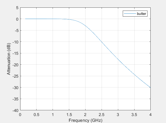
Figure 1. Butterworth filter’s frequency response.

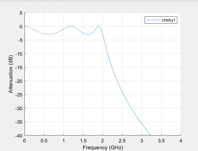
Figure 2. Chebyshev I-type filter’s frequency response.

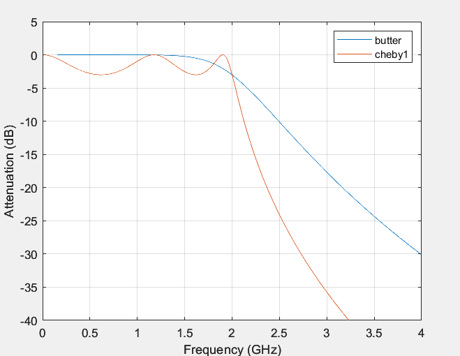
Figure 3. Comparison of the two kinds of filter.

From the frequency response (Figure 3), it can be concluded that the amplitude frequency characteristics of the Butterworth filter are monotonically dropping and smooth in the passband, at the same time those of the Chebyshev I-type filter fluctuate in the passband and are monotonous in the stopband. Firstly, the transition bandwidth and the cutoff frequency of the passband indicate that that of the Butterworth filter with regard of frequency is smooth and without ripples in the transition bandwidth, whereas the transition bandwidth of the Chebyshev I-type filter behaves with ripples in the frequency response. The frequency at which the filter begins to deteriorate within the passband is known as the cutoff frequency [9], and both have a cutoff frequency of 2GHz. Similarly, the attenuation of both filters δ all are 3dB. This indicates that the Butterworth filter can better preserve the original waveform of the signal, and it can be more convenient and easier to process the signal in the later stage. The third contention is that the Butterworth filter’s passband attenuation is the slowest, that is, within the frequency range after the cut-off frequency, the attenuation rate of the filter is relatively small. In contrast, the Chebyshev I-type filter exhibits faster attenuation within the passband range. This means that the Chebyshev I-type filter can provide better suppression in narrower frequency bands.

Given the same order, passband ripple, and edge frequency, Chebyshev Type I filters typically exhibit steeper attenuation characteristics than Butterworth filters. Therefore, before selecting a filter, it is not only necessary to consider actual needs and design requirements, but also to weigh the characteristics of different filters. When there is a high demand for passband ripple, which requires a flatter frequency response, then Butterworth may be a better choice.

Transition width

Compare the transition band widths between the passband and stopband of two types of filters through Figure 3. It can be concluded that compared to the Chebyshev I filter, the attenuation of the transition band of the Butterworth filter is very slow, while the Chebyshev I filter decays very quickly in the passband range, and the transition band bandwidth is very short, which means it can provide a good suppression ability of ten percent. If a filter with strong suppression ability is needed, the Chebyshev I filter is better than the Butterworth filter.

However, compared to the Chebyshev Type I filter, the transition bandwidth is very short. If there is a higher requirement for the transition bandwidth, which requires a smoother transition bandwidth, then the Butterworth filter may be more suitable. The transition bandwidth of the Butterworth filter is smooth and without ripples. So the Butterworth filter at this time is more suitable.

Design complexity

From Figure 1, it can be seen that due to the excessively smooth passband and stopband of the Butterworth filter, as well as slow attenuation in the transition band, these characteristics are not easy to achieve, so more circuit components are needed for design. Similar to Chebyshev filters, it has a variety of filters. It is not only a long transition band with high distortion potential, but it also has consistent amplitude-frequency characteristics both inside and outside the passband. The signal always demonstrates a certain dispersion in the first cycle when the Butterworth filter is being emulated in MATLAB. The amplitude frequency characteristics, however, are quite complete in the future. The Chebyshev Type I filter is relatively simple with low design and calculation costs, while the Butterworth filter is relatively complex with relatively high design and calculation costs.

Filter order

The total amount of second-order filters in a filter is commonly referred to as its order. The filter’s influence on the input signal increases with order [10], This ultimately ends up in a steeper frequency response curve for the filter and a narrower cutoff frequency transition band. Therefore, the higher the order, the better the performance of the filter, but the design and implementation are also more complex, and the computational complexity also increases. Compare by changing the order of the two filters. In this article, it will choose three filter orders: N=2(Figure 4), N=5(Figure 5), N=8(Figure 6):

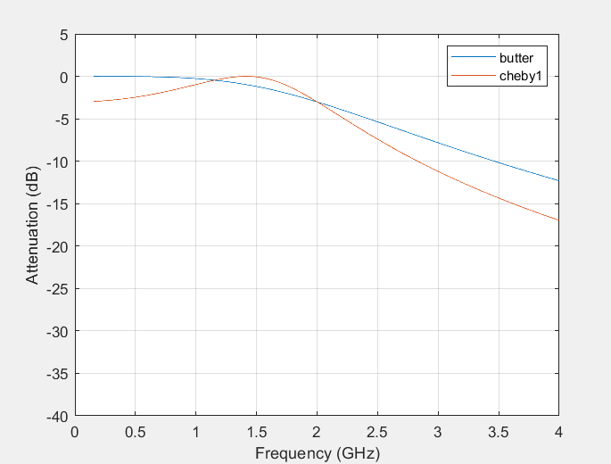
Figure 4. Filter order N=2.

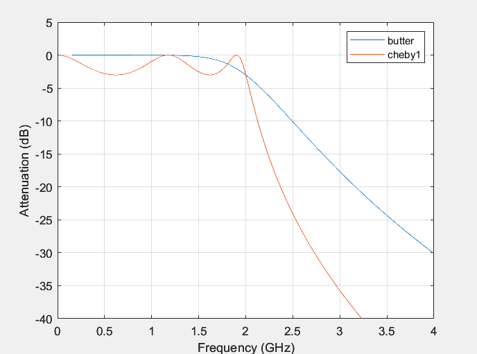
Figure 5. Filter order N=5.

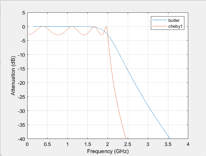
Figure 6. Filter order N=8.

Through comparison, it is found that in general, Chebyshev filters have a lower order and are relatively easier to implement; The Butterworth filter has a higher order and can achieve higher filtering characteristics.

Target application

In engineering, the order of the filter selection needs to be determined based on specific application requirements [11]. Choosing the appropriate order requires balancing the relationship between filter performance and computational complexity. In general, the order of the filter can be determined based on the following factors:

Bandwidth and cut-off frequency

If high-frequency noise needs to be filtered, high-order filters need to be selected to achieve better performance. On the contrary, if low-frequency noise needs to be filtered, a low-order filter can be chosen.

Signal quality requirements

If a high signal-to-noise ratio is required for the output signal, a high-order filter needs to be selected. Because higher-order filters can provide better suppression, thereby reducing noise in the signal [12].

Computational complexity

Higher order filters have higher computational complexity and require more computational resources and processing time. Therefore, in engineering, it is necessary to choose the appropriate filter order based on the system’s computing resources and real-time requirements.

Filter stability

The higher the order of the filter, the less stable it will be. Therefore, when selecting the order of the filter, it is necessary to pay attention to the stability of the filter.

Conclusions

This paper mainly compares the applications and advantages of Chebyshev filter and Butterworth filter. When comparing these two filters, we mainly focus on the following aspects: frequency response, transition band width, filter order, design complexity, and target application. Firstly, we introduced the formulas and related introductions of Chebyshev filter and Butterworth filter. Then, we implemented the code for these two filters separately. When comparing the applications of two types of filters, we mainly compare the following parameters: Frequency response: Chebyshev filters usually have ripples in the passband and flat stopband; Butterworth filters typically have flat passbands and ripple stops. Transition band width: Chebyshev filters have a narrow transition band width and are suitable for applications that require steeper filtering characteristics; And the Butterworth filter has a wider width in the transition band, which is suitable for applications with less strict requirements on the characteristics of the transition band. Filter order: Generally, Chebyshev filters have a lower order and are relatively easier to implement; The Butterworth filter has a higher order and can achieve higher filtering characteristics. Design complexity: Chebyshev filters are relatively simple and have low design and computational costs; And the Butterworth filter is relatively complex, with high design and calculation costs. Target application: Chebyshev filters are suitable for applications with high frequency response requirements, such as communication systems; Butterworth filters are suitable for applications that require flat passbands and wide stopbands, such as audio systems. By comparing the above parameters, it can further analyze and evaluate the application advantages and limitations of Chebyshev and Butterworth filters in different situations. Overall, the choice of filter depends on the specific application scenario and requirements.

References

[1]. Jamalabadi A Y M. Analytical study of magnetohydrodynamic propulsion stability. Journal of Marine Science and Application,2014,13(3).
[2]. Mandal S,Ghoshal P S,Kar R, et al.Optimal Linear Phase Finite Impulse Response Band Pass Filter Design Using Craziness Based Particle Swarm Optimization Algorithm. Journal of Shanghai Jiaotong University (Science),2011,16(06):696-703.
[3]. Wei Yewen, Li Yingzhi, Cao Bin, et al. Research on Low Power Consumption and Energy Balance Technology of Lithium Batteries with Buck Circuit. Journal of Electrical Technology, 2018,33 (11): 2575-2583.
[4]. Liu Yan, Zhang Suying. The ground states and pseudo textures of rotating two component Bose - Einstein condensates trapped in harmonic plus quartz potential. Chinese Physics B, 2016,25 (09): 223-230
[5]. Chiacchiari L,Loprencipe G.Measurement methods and analysis tools for rail irregularities:a case study for urban tram track. Journal of Modern Transportation,2015,23(02):137-147.
[6]. Yang Ziwen, Zhang Zijian, Zhu Yanmeng, et al. Design of bandpass filters for power supply and communication multiplexing circuits. Magnetic Materials and Devices, 2021,52 (05): 79-83.
[7]. Gao S,Xue B,Li J, et al. High-resolution data acquisition technique in broadband seismic observation systems. Science China Technological Sciences,2016,59(6).
[8]. Ye Zhan Design and Implementation of Programmable Gain Amplifiers and Current Mode Complex Bandpass Filters. Southeast University, 2015.
[9]. Mayashi Performance Analysis and Optimization of Filtering Multi tone Modulation System. Chongqing University of Posts and Telecommunications, 2017.
[10]. Xing Y, Lv C, Chen L, et al. Advances in Vision-Based Lane Detection: Algorithms, Integration, Assessment, and Perspectives on ACP-Based Parallel Vision. IEEE/CAA Journal of Automatica Sinica,2018,5(03):645-661.
[11]. MENG B, XU H, RUAN J, et al.Theoretical and experimental investigation on novel 2D maglev servo proportional valve. Chinese Journal of Aeronautics,2021,34(04):416-431.
[12]. Two examples of using physical mechanics approach to evaluate colloidal stability. Science China (Physics,Mechanics & Astronomy),2012,55(06):933-939.
Cite this article
Li,Z. (2024). Chebyshev filter and Butterworth filters: Comparison and applications in different cases. Applied and Computational Engineering,38,102-111.
Data availability
The datasets used and/or analyzed during the current study will be available from the authors upon reasonable request.
Disclaimer/Publisher's Note
The statements, opinions and data contained in all publications are solely those of the individual author(s) and contributor(s) and not of EWA Publishing and/or the editor(s). EWA Publishing and/or the editor(s) disclaim responsibility for any injury to people or property resulting from any ideas, methods, instructions or products referred to in the content.
About volume
Volume title: Proceedings of the 2023 International Conference on Machine Learning and Automation
© 2024 by the author(s). Licensee EWA Publishing, Oxford, UK. This article is an open access article distributed under the terms and
conditions of the Creative Commons Attribution (CC BY) license. Authors who
publish this series agree to the following terms:
1. Authors retain copyright and grant the series right of first publication with the work simultaneously licensed under a Creative Commons
Attribution License that allows others to share the work with an acknowledgment of the work's authorship and initial publication in this
series.
2. Authors are able to enter into separate, additional contractual arrangements for the non-exclusive distribution of the series's published
version of the work (e.g., post it to an institutional repository or publish it in a book), with an acknowledgment of its initial
publication in this series.
3. Authors are permitted and encouraged to post their work online (e.g., in institutional repositories or on their website) prior to and
during the submission process, as it can lead to productive exchanges, as well as earlier and greater citation of published work (See
Open access policy for details).