Breast cancer prediction based on the machine learning algorithm LightGBM

Jiayu Zhu

Introduction

The breast cancer is a significant threat to the modern people’s health. Many factors could lead to a risk of breast cancer, such as alcohol abusing and exposing to radiation [1]. As a widely known fact, that the earlier a cancer is found, the better the treatment’s effect will be. If there is a misdiagnosis, the patient would lose the best time for treatment, which will lead to horrible consequences [2]. Therefore, the diagnosis precision and self-diagnosing would be very important in the prevention of breast cancer. An Artificial Intelligence (AI) model that enables a quick prediction of breast cancer could be of great help. In hospitals, the AI model could offer a reliable reference to the doctors, which could effectively enhance diagnosis accuracy. With an AI diagnosis device, people could diagnose themselves at home, which provides a convenient self-diagnosing method.

To realize an AI diagnosis model, researchers are actually doing ‘Data Mining’, which is trying to dig out useful but not intuitive information from a big load of data [3]. Many researchers showed great inclination toward doing data mining, for there exists a great amount of data, and there lies enormous potential value in these data [3]. In the prediction of breast cancer, prior researchers applied various algorithms, and constructed many methods to optimize the performance of the model [3]. For instance, Islam et al. utilized both the Artificial Neural Network (ANN) and some machine learning methods to do a comparative experiment. They concluded that the ANN performed the best in all methods, and the Support Vector Machine (SVM) algorithm performed the best in the traditional machine learning methods [4]. There are researchers like Haifeng Wang et al. who got a very high accuracy, that is 97.83%, by applying delicate data-preprocessing on the usually low-accuracy Bayes algorithm [5]. M. S. Yarabarla et al. investigated the data of machine-learning cancer prediction in medical reality [6]. They concluded that the SVM is now the most welcomed machine-learning method in cancer prediction, for its high accuracy and low financial cost. They also compared a similar algorithm to SVM, that is the Relevance Vector Machine (RVM), and found out that the RVM and SVM are both widely applied in actual medical scenarios, but in different situations.

In this study, the author applies one of the most focused traditional machine-learning methods, that is the Light Gradient Boosting Machine (LightGBM) algorithm, on the prediction of breast cancer. In the experiment of the code, the input data is pre-processed by dividing the dataset into training set and testing set, and that is the only data-preprocessing applied in the study. The LightGBM algorithm has many merits in the job of classification. It is well-known for high accuracy, high speed and small storage cost. These merits excellently meet the needs of medical application. The LightGBM is also capable of processing huge data, which meets the needs of actual medical scenarios. In the code experiment, the LightGBM algorithm is evaluated in accuracy, time cost, Area under Curve (AUC) and confusion matrix. The result of the experiment shows that the LightGBM algorithm has a satisfying performance, which means the LightGBM algorithm is very suitable for cancer prediction. However, its sensitivity to over-fitting shows that it needs a cautious hyper-parameter adjusting.

Methodology

Dataset description and preprocessing

In this paper, the author conducts the experiment on the dataset ‘The Breast Cancer Prediction Dataset’ from Kaggle [7]. The dataset includes 569 data samples. Each sample has 6 attributes, that are the mean radius, the mean texture, the mean perimeter, the mean area, the mean smoothness and the diagnosis. For the feature ‘diagnoses, if a sample represents a breast cancer patient, the feature’s value is 1, otherwise the feature’s value is 0. And there are 212 samples (37.3%) that represent breast cancer patients, and 357 samples (62.7%) that represent healthy people. The data-preprocessing in the study simply aims to fit the input data into the model, and the dataset the study chose is already delicate enough before any optimization. Hence there’s only one step in the data-preprocessing, that is dividing the dataset into training set and testing set, with a proportion of 70 percent and 30 percent respectively.

Proposed approach

The study aims to find a classifier that has good comprehensive performance. However, the accuracy of the classifier is primarily focused. As Fig.1 illustrates, the incipient LightGBM classifier is firstly optimized by adjusting hyper-parameters. By decreasing the upper bound of each decision tree’s depth and the quantity of leaves in each decision tree, a reduction of the over-fitting problem can be observed on the AUC line. The classifier is then optimized again by applying the bootstrap aggregating (Bagging) method. The study applies the Bagging method since the LightGBM algorithm is sensitive to over-fitting, and the method can reduce the occurrence of over-fitting significantly. The Bagging method divides the input dataset into many small datasets, and trains different models on these datasets separately. The variance of the classifier is thus reduced, which prevents the occurrence of over-fitting. After all the optimizing processes, the input data is fed into the classifier. All three versions of the classifiers are evaluated on the comprehensiveness of different metrics. In detail, the metrics are the AUC, the accuracy and the confusion matrix.

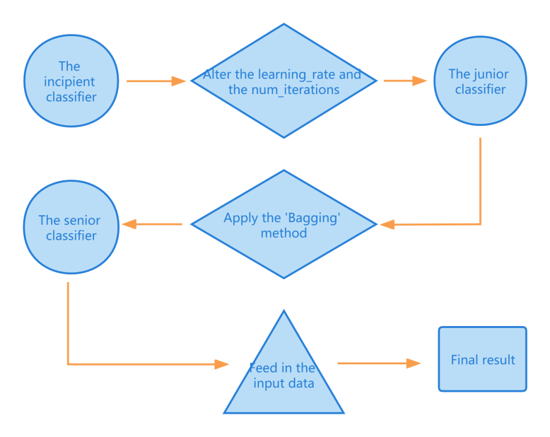
Figure 1. Illustration of the whole process.

LightGBM. The LightGBM algorithm is a frame of the Gradient Boosting Decision Tree (GBDT) model. Before LightGBM, the canonical method of GBDT was the Extreme Gradient Boosting (XGBoost) algorithm. The LightGBM can be viewed as an optimized version of the XGBoost in speed, accuracy and storage cost. Traditionally, LightGBM utilizes a method names ‘Gradient-based One-Side Sampling’(GOSS) at the beginning to reduce the over-fitting problem. Since GOSS is not used with Bagging together, the study didn’t apply the GOSS method.

To start with, the feature values are processed by a method called ‘Histogram algorithm’. In the Histogram algorithm, the eigenvalues of the input data are converted into k discrete integers [8]. Compared to the traditional ‘pre-sorted algorithm’ applied in the XGBoost algorithm, the space complexity of the histogram algorithm decreases from O(#data*#feature) to O(k*#feature), while k<<#data. After the feature values are discretized, LightGBM applies a method to decrease the time cost, that is the Exclusive Feature Bundling (EFB). The basic theory of the EFB is that many features in the feature space are exclusive [9]. ‘Exclusive’ means the features are seldom non-zero simultaneously, and it is harmless to bundle the exclusive features together [9]. By utilizing the EFB, the time complexity of building the histogram decreases from O(#data×#feature) to O(#data×#bundle), while #bundle<<#feature. After the EFB, it comes to the phase of growing decision trees. The XGBoost algorithm utilizes the ‘level-wise’ strategy. As Fig.2 shows, it splits all the previous leaves when growing new leaves [10]. In this strategy, some nodes with small information gain are also split into new leaves, which leads to resource waste and big time-cost [8]. In the LightGBM algorithm, a new strategy called ‘leaf-wise’ is utilized. In the leaf-wise strategy, as Fig.3 illustrates, only those leaves with the biggest information gain are split into new leaves [8]. This new strategy significantly reduces the time cost of the algorithm, for it traverses much fewer nodes when growing decision trees.

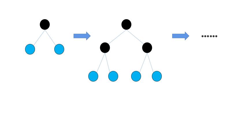
Figure 2. Demonstration of level-wise growth.

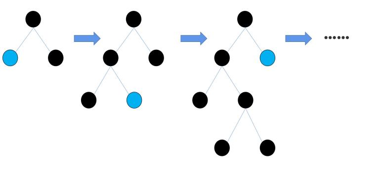
Figure 3. Demonstration of leaf-wise growth.

Conclusively, the sequence of the steps in the LightGBM algorithm in the study is shown in Fig.4. The LightGBM serves as the core model in this study. LightGBM provides an accurate, highly efficient classifier for the cancer prediction task, which enables the data-mining process on the breast cancer dataset.

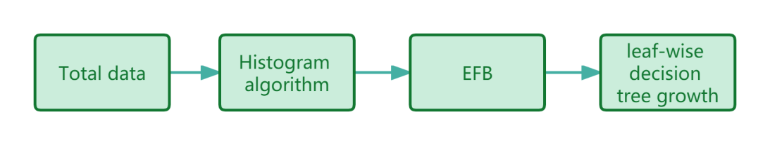
Figure 4. The sequence of steps in the LightGBM algorithm in the study.

Bagging. The Bagging method aims to reduce the variance of the classifier, and thus reduce the occurrence of over-fitting. It firstly does the process of ‘bootstrap’, that is sampling with replacement. For k (k is any positive integer) rounds of ‘bootstrap’, k training sets are formed. After that, k different models are trained on these training sets separately. Finally, these different models combine as one model, and the task of classification is conducted on this one model. The variance of the model can be significantly reduced due to the following mathematical properties of variance,

\(Var(cX) = c²Var(X).()\) (1)

where c is a constant, “Var()” means “the variance of”, and “c²” represents the square of c.

\(Var(X1 + \cdot \cdot \cdot + Xn) = Var(X1) + \cdot \cdot \cdot + Var(Xn).()\) (2)

Therefore, the variance of the combined model is as follows:

\(Var(\frac{1}{n}\sum_{i = 1}^{n}X_{i}) = \frac{1}{n²}Var(\sum_{i = 1}^{n}X_{i}) = \frac{Var(X_{1}) + \cdot \cdot \cdot + Var(X_{n})}{n²}.()\) (3)

While training the different models, some of the models might have big variances. As formula (3) shows, these big variances are neutralized by other models’ variances in the variance of the combined model. In LightGBM, the idea of ‘Bagging’ is reflected in the fact that the classification is based on the comprehensiveness of many independent decision trees. The user is applying the Bagging method as long as he or she is using LightGBM, even if the user doesn’t set Bagging-related hyper-parameters. In order to enhance the Bagging method’s ability on reducing over-fitting, a certain proportion of data instances can be discarded in every round’s Bagging (the proportion is defined by setting the Bagging-related hyper-parameters). The Bagging method in the study serves as a solution to LightGBM’s over-fitting sensitivity.

Implemented details

The study utilized Python 3.10.12 and the lightgbm package to implement the LightGBM model. To implement the bagging method, the study used the Scikit-learn library. For data visualization, the study used the Seaborn and the Matplotlib libraries. The code experiment in the study is conducted on a HP Zhan device with an AMD Ryzen CPU. For the setting of hyper-parameters, the study conducted the experiment on three sets of hyper-parameters, that are: default, ‘upper-bound of each decision tree’s depth =3, quantity of leaves in each decision tree =7’and ‘upper-bound of each decision tree’s depth =3, quantity of leaves in each decision tree =7, the frequency of bagging =4, proportion of instances retained in every round’s bagging=0.2’. The adjusting of the hyper-parameters aims to reduce the over-fitting problem without hurting the accuracy on testing data.

Result and discussion

By the evaluation and visualization of the incipient and the optimized LightGBM model, the study shows that LightGBM is an accurate and fast model, but quite sensitive to over-fitting. To start with, the AUC line of the incipient classifier is shown in Fig.5. The incipient classifier is the LightGBM classifier with default hyper-parameters, and doesn’t use the Bagging method. The Fig.5 reveals that although the AUC of both the training set and the testing set are very high, the over-fitting problem is obvious, because there’s a big difference between the AUC on training set and the AUC on testing set.

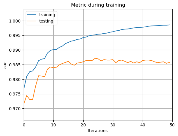
Figure 5. The AUC line of the incipient classifier.

To cope with the over-fitting problem, the junior classifier is worked out by adjusting the hyper-parameters. In detail, two hyper-parameters are set as follows: upper-bound of each decision tree’s depth =3, quantity of leaves in each decision tree =7. As is shown in Fig. 6, the problem of over-fitting is significantly reduced. The reason for the reduction of the over-fitting problem in the first optimization is as follows: After the hyper-parameters are altered, the max depth and the number of leaves of the decision trees are restricted. Therefore, the model’s structure becomes simpler, and a simple structure model has little inclination to have over-fitting problem. However, over-fitting still exists, and gets worse as ‘iterations’ grows.

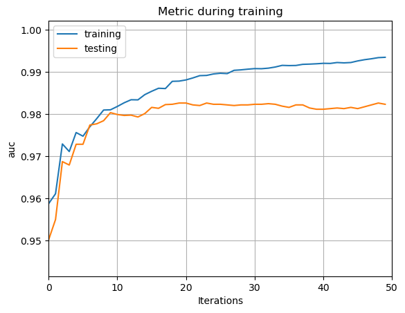
Figure 6. The AUC line of the junior classifier.

To eliminate the problem of over-fitting, the classifier still needs an optimization. Therefore, the senior classifier is worked out by applying the Bagging method and adjusting hyper-parameters. Fig. 7 shows the AUC line of the senior classifier. The hyper-parameter is set as: upper-bound of each decision tree’s depth =3, quantity of leaves in each decision tree =7, the frequency of bagging =4, proportion of instances retained in every round’s bagging=0.2. Fig. 7 shows that the over-fitting problem is well handled in the senior classifier. The reason for the reduction of the over-fitting problem in the second optimization is as follows: After the Bagging method is applied, some of the training data is discarded while training the model. Therefore, the model can only have an incomplete knowledge of the training set. This leads to a simpler structure of the model, which reduces the emergence of over-fitting.

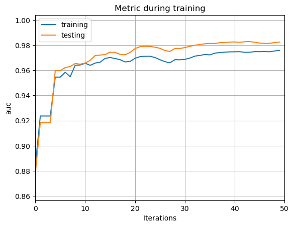
Figure 7. The AUC line of the senior classifier.

After the over-fitting problem is discussed, this section focuses on the accuracy of the classifiers. The accuracies of 3 versions of classifiers are shown in Table 1. Table 1 shows that all the 3 versions of LightGBM classifiers have a high accuracy of over 90%. By altering the hyper-parameters and applying the Bagging method, the accuracy on the training set declines, while the accuracy on the testing set stays stable. The decline in the accuracy on the training set can be attributed to the same reason as the reduction in over-fitting. Firstly, after the hyper-parameters are adjusted, the structure of the LightGBM becomes simpler, and a simpler model tends to have a lower accuracy. Secondly, after the Bagging method is applied, the model can only have an incomplete knowledge of the training set, which leads to a lower accuracy in the prediction on training set.

Table 1 also shows the time cost of the three versions of classifiers. Table 1 reveals that all three versions of the LightGBM classifiers have a small time-cost of under 0.5s. This is a manifestation of the LightGBM’s high speed. And the time cost declines as the model is optimized. This can be attributed to the simplification of the structure of the model.

Table 1. Accuracy of Different LightGBM Classifiers.

In order to have a meticulous evaluation of the model’s performance, the confusion matrixes of the three versions of classifiers are plotted. As Fig. 8 and Fig. 9 show, the classifiers made precise predictions on both the positive and negative instances. The result in the confusion matrix manifests that the classifiers have good performance on both the positive and negative instances.

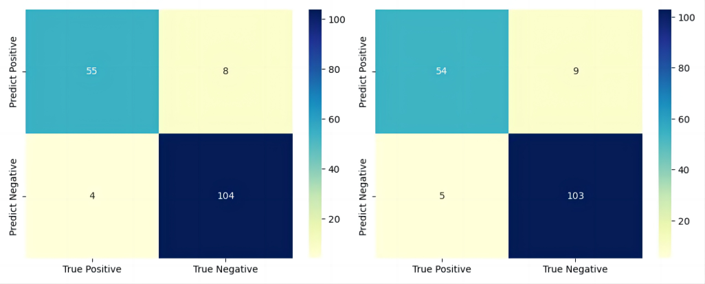
Figure 8. Left: the confusion matrix of the incipient classifier. Right: the confusion matrix of the junior classifier.

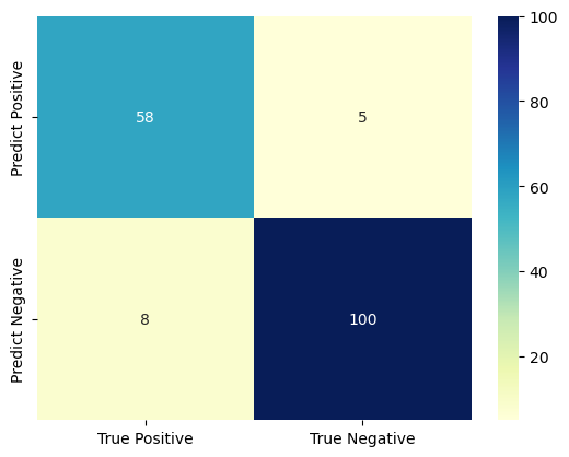
Figure 9. The confusion matrix of the senior classifier.

The mentioned results in the study can serve as an enlightenment on the application of LightGBM in actual medical scenarios. Firstly, it reveals that LightGBM is a model with high accuracy and high speed. LightGBM is also a traditional machine-learning model, which means LightGBM doesn’t need to work on a device with an advanced GPU. People only need a device with a normal CPU to process the LightGBM model. Therefore, LightGBM can be utilized in designing a portable, cheap and accurate device which helps people measure their health condition at home. LightGBM can also help impoverished areas realize accurate medical detection. Secondly, LightGBM is a model sensitive to over-fitting. While programming a medical device on LightGBM, the hyper-parameters should be cautiously adjusted based on the application reality. Methods like Bagging should also be considered to cope with the over-fitting problem.

Conclusion

This study constructs the LightGBM algorithm to realize breast cancer prediction. LightGBM meets the need for medical reality well due to its high accuracy, high speed and low financial cost. In addition, the study adjusts hyper-parameters and Bagging to cope with the over-fitting problem. The study finds that LightGBM has great potential in medical detection, but programmers should handle its over-fitting sensitivity cautiously. For future work, the study will focus on constructing models based on deep-learning algorithms. Models based on deep-learning algorithms will be far more accurate than traditional machine-learning models. Meanwhile, since the deep-learning models tend to have big time cost and big financial cost, the study will try to get a relatively fast and cheap model by optimizing the model on many metrics.

References

[1]. Huang M W Chen C W Lin W C Ke S W Tsai C F 2017 SVM and SVM ensembles in breast cancer prediction PloS one 12(1): p e0161501
[2]. Islam M M Haque M R Iqbal H Hasan M M Hasan M and Kabir M N 2020 Breast cancer prediction: a comparative study using machine learning techniques SN Computer Science 1: pp 1-14
[3]. Li Y and Chen Z 2018 Performance evaluation of machine learning methods for breast cancer prediction Appl Comput Math 7(4): pp 212-216
[4]. Islam M M Haque M R Iqbal H Hasan M M Hasan M and Kabir M N 2020 Breast cancer prediction: a comparative study using machine learning techniques SN Computer Science 1: pp 1-14
[5]. Wang H and Yoon S W 2015 Breast cancer prediction using data mining method IIE Annual Conference. Proceedings. Institute of Industrial and Systems Engineers (IISE) 818
[6]. Yarabarla M S Ravi L K and Sivasangari A 2019 Breast cancer prediction via machine learning. international conference on trends in electronics and informatics (ICOEI) IEEE pp 121-124
[7]. MERISHNA SINGH SUWAL Breast Cancer Prediction Dataset Kaggle 2018 https://www.kaggle.com/datasets/merishnasuwal/breast-cancer-prediction-dataset
[8]. Zhang D and Gong Y 2020 The comparison of LightGBM and XGBoost coupling factor analysis and prediagnosis of acute liver failure IEEE Access 8: pp 220990-221003
[9]. Ke G Meng Q Finley T 2017 Lightgbm: A highly efficient gradient boosting decision tree Advances in neural information processing systems 30
[10]. Al Daoud E 2019 Comparison between XGBoost, LightGBM and CatBoost using a home credit dataset International Journal of Computer and Information Engineering 13(1): pp 6-10
Cite this article
Zhu,J. (2024). Breast cancer prediction based on the machine learning algorithm LightGBM. Applied and Computational Engineering,40,77-84.
Data availability
The datasets used and/or analyzed during the current study will be available from the authors upon reasonable request.
Disclaimer/Publisher's Note
The statements, opinions and data contained in all publications are solely those of the individual author(s) and contributor(s) and not of EWA Publishing and/or the editor(s). EWA Publishing and/or the editor(s) disclaim responsibility for any injury to people or property resulting from any ideas, methods, instructions or products referred to in the content.
About volume
Volume title: Proceedings of the 2023 International Conference on Machine Learning and Automation
© 2024 by the author(s). Licensee EWA Publishing, Oxford, UK. This article is an open access article distributed under the terms and
conditions of the Creative Commons Attribution (CC BY) license. Authors who
publish this series agree to the following terms:
1. Authors retain copyright and grant the series right of first publication with the work simultaneously licensed under a Creative Commons
Attribution License that allows others to share the work with an acknowledgment of the work's authorship and initial publication in this
series.
2. Authors are able to enter into separate, additional contractual arrangements for the non-exclusive distribution of the series's published
version of the work (e.g., post it to an institutional repository or publish it in a book), with an acknowledgment of its initial
publication in this series.
3. Authors are permitted and encouraged to post their work online (e.g., in institutional repositories or on their website) prior to and
during the submission process, as it can lead to productive exchanges, as well as earlier and greater citation of published work (See
Open access policy for details).