1.Introduction

Space debris in low earth orbit (LEO) and geosynchronous equatorial orbit (GEO) are mostly the fragments from resident space objects (RSO), i.e., human-made satellites, discard rocket bodies and tiny pieces from the collision among other debris. Tracking active and inactive satellites and space debris is one of main missions in Space situation awareness (SSA), a space surveillance system was initiated by ESA [1]. By 2021, more than 1 million of space debris for sizes from larger than 1cm to 10cm on earth orbit was estimated by ESA’s space debris office [2] and over 68,000 space objects were tracked and catalogued by ESA util July, 2020 [3]. Distinguishing between active satellites and space debris heavily relies on understanding the RSO population. Space debris classification plays a vital role in collision avoidance and debris removal mission [4]. These efforts are aimed at safeguarding the valuable space assets and maintaining the safe of the space environment.

There are many ways to detect space objects and space debris, including camera, optical sensor and radar system in the ground. Classification of RSOs is the main mission and a key challenge of the SSA program which has many applications. By utilizing ground-based radars, optical telescopes, and laser systems, its aim is to detect, observe, and classify objects that are larger than 5–10 cm in LEO – the most densely populated orbital area. Similarly, for higher orbits such as the Medium and Geostationary Earth Orbits (MEO) and GEO, the focus is on objects larg0er than 0.3–1.0 m. Radar observations are the most feasible method for examining the space debris environment on LEO, particularly for objects exceeding 1 cm in size [5]. Moreover, radar system continues to serve as a significant space object classification way at today due to the cheap prices of manufacturing. RCS, as one crucial physical characteristic of radar target, provides information about the type of the SO. As a result, radars capable of measuring the RSO’s characteristics are helpful to catalogue the RSO based on RCS [6].

Recent progress in machine learning (ML) and deep learning (DL) are utilized in many applications, such as data classification, image processing and patterns identification. The ability of ML and DL methods to identify and classify RSOs (debris/non-debris problem) based on sky observation and catalogue information has been demonstrated in several studies. Roberto Furfaro et al evaluated the Deep Meta-Learning’s (DML) potential application in SSA [7]. Mahmoud Khalil et al utilized several ML methods, feature extraction and oversampling techniques to improve the performance of the classifier via light curves of RSOs [8].

RCS data also have been widely utilized in previous work for the RSO classification and identification. Nevertheless, there are one tricky problem, an RSO’s RCS data influenced by various factors, such as its shape, motion, angular velocity, atmospheric conditions, altitude, material, and the characteristics of the radar [9]. Resolving this issue is a challenge topic, because of its physical complexity, Cai Wang et al using the k-nearest neighbor (KNN) fuzzy classifier to accomplish the object identification [10]. In Reference [9], statistical features, size features and altitude ability features were extracted from RCS sequences by Jin Sheng et al. The Greedy algorithm was used by Xuehui Lei et al with the extracted statistical features [11]. Hence, applying machine learning methods on RCS in real-world may offer a confidential approach.

In this study, in the context of RSOs classification (debris or non-debris) based on RCS, we investigate the application of several supervised machine learning (classification techniques) [12], including Logistic Regression, Naive Bayes, K- Nearest Neighbor (KNN), Support Vector Machine (SVM), etc. Given that the numerous features of RSOs in the dataset from ESA, these ML classification models are trained based on RCS with the selected features set. Meanwhile, we evaluate their performance by the Accuracy (Acc), Precision (Pre) and Recall (Rec). The dataset employed in this study also encounters the Class-imbalance problem (the proportion of space debris to non-debris is roughly 5 to 1). To tackle this challenge, we are exploring the utilization of three oversampling approaches, i.e., Synthetic Minority Oversampling Technique (SMOTE) [13], synthetic minority oversampling technique-support vector machine (SMOTE-SVM) [14] and Adaptive Synthetic Sampling (ADASYN) [15]. The different ML classifiers’ performance is examined to pinpoint the most proper oversampling method.

The arrangement of the research as follows: Section 2 details the overview of the dataset and the selection of features. Section 3 introduces several machine learning classification and oversampling techniques. Section 4 offers a concise summary of the implement environment and t observations and findings are presented in the second half. Finally, Section 5 encapsulates the conclusions drawn from the study.

2.Data Overview and Preparation

2.1.Data Overview

The dataset from ESA’s Database and Information System Characterizing Objects in Space (DISCOS) is consisted of 10,119 resident space objects with 16 features, which contains 8,432 space debris, 1,362 payloads, 217 rocket bodies and 108 TBA objects, until 2020. The existing dataset comprises 9,179 Resident Space Objects (RSOs), each associated with a single RCS (Radar Cross Section) data point. These 9,179 RSOs are categorized into distinct classes: the non-debris class, which comprises 1530 objects, and the debris class, which encompasses the remaining 7,649 objects. This distribution results in a class ratio of 5:1, with a larger representation in the non-debris class compared to the debris class.

2.2.Features selection

When working with the sixteen features of RSOs for the classification of RSOs, it's important to address redundant features as they can diminish the classification performance. Therefore, to enhance computational efficiency and achieve effective RSOs classification, it becomes essential to choose meaningful features.

A straightforward and common criterion for feature selection is the correlation heatmap, which computes and displays the correlation coefficient\( {ρ_{x,y}} \)between two random variables\( X \)and\( Y \). The correlation coefficient\( {ρ_{X,Y}} \)is defined by the formula as below,\( {μ_{X}} \)and\( {μ_{Y}} \)are expected values and\( {σ_{X}} \)and\( {σ_{X}} \)are standard deviations.

\( {ρ_{x,y}}=\frac{Cov(X,Y)}{{σ_{X}}{σ_{Y}}}=\frac{E[(X-{μ_{X}})(Y-{μ_{Y}})]}{{σ_{X}}{σ_{Y}}}, if {σ_{X}}{σ_{Y}} \gt 0. \)(1)

The correlation heatmap displays the correlation coefficient among all statistical features of the RSO in the dataset, as the figure 1.

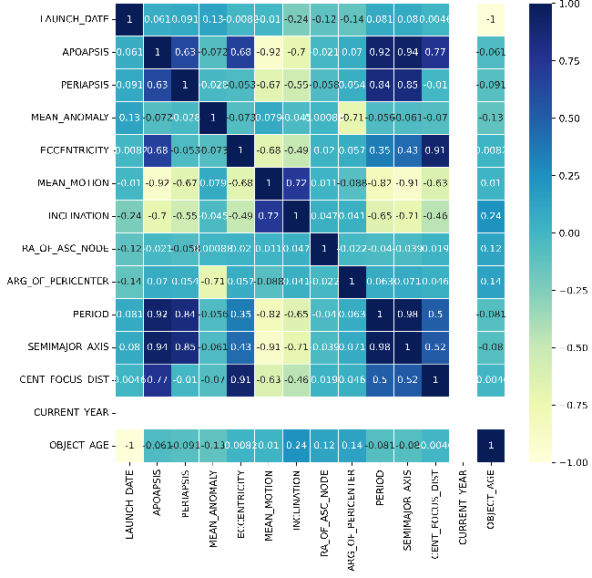
Figure 1. Correlation between Features.

According the Figure 1, 9 features which have strong correlation (the value of correlation efficient\( ρ \gt 0.6 \)) with other features are chosen from previous features space, i.e., ‘OBJECT_TYPE’, ‘CENT_FOCUS_DIST’, ‘APOAPSIS’, ‘MEAN_MOTION’, ‘INCLINATION’, ‘ECCENTRICITY’, ‘SEMMAJOR AXIS’, ‘PERIOD’ and ‘RCS_SIZE’. As a result, the selected features set has 9 dimensions.

The precise definition of the selected features as the table 1.

Table 1. Description of Selected Features in the Satellites and Debris in Earth’s Orbit Dataset.

3.Methodologies

In this research, we construct the selected features set of RSOs from the dataset in Section 2. In Section 3, we will utilize three oversampling strategies to solve the Class-imbalance problem in the dataset and experiment on the combination of seven ML classifiers with different oversampling technologies.

3.1.Oversampling Strategies

As noted earlier, the dataset displays a significant class imbalance which can influence the ML algorithms realization and potentially causing the bias in the space debris class. Hence, in order to address this issue, oversampling techniques were utilized which insert synthetic instances into the minority class. Three oversampling techniques were employed in this paper, i.e., Synthetic Minority Oversampling Technique (SMOTE), synthetic minority oversampling technique-support vector machine (SMOTE-SVM) and Adaptive Synthetic Sampling (ADASYN).

SMOTE's core concept involves the identification of the k-nearest neighbors (KNN) for each minority class sample. Subsequently, synthetic data points are inserted by connecting these points with lines. The process iterates by randomly selecting minority data points until a balanced distribution is attained, aligning the minority and majority class sizes.

SMOTE-SVM, unlike KNN-based oversampling techniques, doesn’t identify the borderline directly. Instead, it focuses on reinforcing the borderline by leveraging Support Vector Machines (SVM).

ADASYN operates on the core principle of generating additional the minority samples, taking into account their distributions. This process leverages the KNN to identify the density distribution associated with all the minority samples. As a result, it introduces a sufficient number of minority samples to harmonize their representation with that of the majority class within that specific distribution.

3.2.Classification Models

•Logistic Regression: A statistical method used for the ML classification. It uses the logistic function to describe the probability of the outcome from the particular class. The formula as below.

\( P(N=1|M)=\frac{1}{1+{e^{-({c_{0}}+{c_{1}}{M_{1}}{+c_{2}}{M_{2}}+…+{c_{n}}{M_{n}})}}} \)(2)

\( P(N=1|M) \)is the probability that the probability that the dependent variable\( N \)belongs to class 1 given the input features\( M \). The coefficients associated with features\( M \)are denoted by\( {c_{n}} \).

•Naive Bayes: A ML classification algorithm via Bayes' theorem. The formula as below.

\( P(N|M)=\frac{P(N) P(MN)}{P(M)} \)(3)

\( P(N|M) \)is the probability of the data point belonging to class,\( P(N) \)is the prior probability of class,\( P(M|N) \)is the probability of observing features (likelihood),\( P(M) \)is the marginal likelihood, the probability of observing features\( M \).

•K- Nearest Neighbour: The straightforward and efficient supervised machine learning algorithm employed in classification analysis without strict formulae. It makes predictions by taking into account either the majority class or the average value of the KNN points within the feature space.

•Support Vector Machine: The robust supervised ML method applied for classification purposes. It is based on the idea that by maximizing this margin, it reduces the risk of overfitting and generalizes well to new, unseen data. SVM is effective for separable data through the application of various kernel functions.

•AdaBoost: The ensemble machine learning method that combines numerous weak learners to produce a robust classifier. It focuses on improving the classification performance by giving more weight to the data points that are misclassified by previous weak classifiers.

•Random Forest Classifier: The ensemble ML method that is used for classification purposes. It serves as an extension of the decision tree method and combines multiple decision trees to enhance the prediction accuracy.

•Perceptron: A Perceptron is a supervised learning algorithm that models a simplified neuron. It takes a set of input data, assigns power weights to these inputs, calculates the sum of data, then processes outcomes through the function. The output of the activation function determines the class to which the input is assigned (usually binary classification: 0 or 1).

4.Implementation and Testing

In this study, all the models were developed within a Python 3.11.2 environment, The hardware setup includes a 5.2GHz i7-13700 CPU, a RTX 4080 GPU, and 16GB of RAM.

4.1.Evaluation Index

In evaluating the performance of these ML classifiers, there are three universal metrics be used for binary classification analysis. (TP: true positive, FP: false positive, TN: true negative, FN: false negative)

•Accuracy (Acc): The proportion of accurate predictions (comprising true positives and true negatives) to the total number of samples assessed, which can indicate the classifier’s capability to identify samples with the positive and negative classes.

\( Acc=\frac{(TP+TN)}{(TP+TN+FP+FN)} \)(4)

•Precision (Pre): The performance argument that measures the accuracy of positive prediction made by the classifier. Pre is aiming to assess the quality that the classifier avoids false positives.

\( Pre=\frac{TP}{(TP+FP)} \)(5)

•Recall (Rec): The performance argument that measures the capability of classifiers to identity all relevant objects from the positive class. Rec can evaluate the classifier’s ability to capture as many positive samples as possible.

\( Rec=\frac{TP}{(TP+FN)} \)(6)

4.2.Classification Performance

The performance (Acc, Pre and Rec score) of seven machine learning classifiers with selected features is represented in Table 2.

Table 2. The performance of the ML method.

Drawing from the investigation of several computational experiment results, we can make the following observations and findings:

•As far as the selection of a particular classifier, the SVM model has the emergence of frequently excellent performance (denoted by bold fonts), regardless of the oversampling methods employed. The peak performance is achieved when SVM with SMOTE-SVM method is employed on the selected features space, resulting in the accuracy of 99.7%, the recall of 99.4 and the precision of 98.7%. Likewise, the SVM model demonstrates outstanding performance in all oversampling strategies.

•When we compare the capability of oversampling techniques, it becomes evident that SMOTE-SVM has the best performance among the oversampling techniques utilized in this paper. The conclusion reinforced by the average performance score (the accuracy of 97.2%, the recall of 88.4% and the precision of 94.3%), regardless of the classifier employed.

5.Conclusion

In this paper, we explore the efficacy of several machine learning techniques when applied to task of RSOs classification via the real-world RCS data. A series of computational experiments are implemented to process the dataset from ESA within the selected features set, which is generated from the correlation heat map. To solve the class-imbalance issue in the dataset which has an approximate ratio of 5:1 between space debris class and non-debris class. Therefore, three oversampling techniques are employed, such as SMOTE, SMOTE-SVM, and ADASYN. Eventually, seven machine learning classifiers, i.e., Logistic Regression, Naive Bayes, KNN, SVM, AdaBoost, Random Forest Classifier and Perceptron are assessed in terms of Acc, Pre and Rec. The SMOTE-SVM oversampling method with the SVM classifier have the best performance (Acc: 99.7%, Pre: 98.7% and Rec: 99.4) among all combinations.

The following work is to investigate the potential of employing deep learning methods and several features extraction methods in comparison to the current feature selection approach. Moreover, there is a need to consider using a larger dataset because of the significant increase of RSOs year by year.

References

[1]. Xiang, Y., Xi, J., Cong, M., Yang, Y., Ren, C., & Han, L. Space debris detection with fast grid-based learning. In 2020 IEEE 3rd International Conference of Safe Production and Informatization (IICSPI). 2020, pp. 205-209.
[2]. Flohrer, T., Lemmens, S., Bastida Virgili, B., Krag, H., Klinkrad, H., Parrilla, E., ... & Pina, F. DISCOS-current status and future developments. In Proceedings of the 6th European Conference on Space Debris. 2013, 723, pp. 38-44.
[3]. McLean, F., Lemmens, S., Funke, Q., & Braun, V. DISCOS 3: An improved data model for ESA’s database and information system characterising objects in space. In 7th European Conference on Space Debris. 2017, 11, pp. 43-52.
[4]. Allworth, J., Windrim, L., Bennett, J., & Bryson, M. A transfer learning approach to space debris classification using observational light curve data. Acta Astronautica. 2021, pp. 301-315.
[5]. Kessler, D. J.. Orbital debris environment for spacecraft in low earth orbit. Journal of spacecraft and rockets. 1991, 28, 3, pp. 347-351.
[6]. Wang, C., Fu, X., Zhang, Q., Jiao, L., & Gao, M. Space object identification based on narrowband radar cross section. In 2012 5th International Congress on Image and Signal Processing, 2022 pp. 1653-1657.
[7]. Furfaro, R., Campbell, T., Linares, R., & Reddy, V. Space debris identification and characterization via deep meta-learning. In First Int’l. Orbital Debris Conf. 2019, pp.1-10.
[8]. Mahmoud Khalil, Elena Fantino, Panos Liatsis, Evaluation of Oversampling Strategies in Machine Learning for Space Debris Detection. In 2019 IEEE International Conference on Imaging Systems and Techniques (IST), 2019, pp. 1-6.
[9]. Cai Wang, Xiongjun Fu, Qian Zhang, Long Jiao, Meiguo Gao, Space Object Identification based on Narrowband Radar Cross Section. In 2012 5th International Congress on Image and Signal Processing, 2012, pp.1653-1657.
[10]. Jin Sheng, Gao Mei Guo, Wang Yang, Technology of space target recognition based on RCS. Modern Radar, 2010, 32, 6, pp.59-62.
[11]. Xuehui Lei, Xiongjun Fu, Cai Wang, Meiguo Gao, 2011, Statistical Feature Selection of Narrowband RCS Sequence Based on Greedy Algorithm. In Proceedings of 2011 IEEE CIE International Conference on Radar, 2011, 2, pp. 1664-1667.
[12]. Aized Amin Soofi, Arshad Awan, Classification Techniques in Machine Learning: Applications and Issues. Journal of Basic & Applied Sciences, 2017, 13, pp. 459-465.
[13]. N. V. Chawla, K. W. Bowyer, L. O. Hall and W. P. Kegelmeyer, SMOTE: Synthetic Minority Over-sampling Technique. Artificial Intelligence Research, 2002, 16, pp. 321-357.
[14]. H. M. Nguyen, E. W. Coope and K. Kamei, Borderline Over-sampling for Imbalanced Data Classification. International Journal of Knowledge Engineering and Soft Data Paradigms, 2009, 3, 1, pp. 4- 21.
[15]. H. He, Y. Bai, E. A. Garcia and S. Li, ADASYN: Adaptive Synthetic Sampling Approach for Imbalanced Learning. In IEEE International Joint Conference on Neural Networks (IEEE World Congress on Computational Intelligence). 2008, pp.1-11.
Cite this article
Zhang,Y. (2024). Machine learning with oversampling for space debris classification based on radar cross section. Applied and Computational Engineering,49,102-108.
Data availability
The datasets used and/or analyzed during the current study will be available from the authors upon reasonable request.
Disclaimer/Publisher's Note
The statements, opinions and data contained in all publications are solely those of the individual author(s) and contributor(s) and not of EWA Publishing and/or the editor(s). EWA Publishing and/or the editor(s) disclaim responsibility for any injury to people or property resulting from any ideas, methods, instructions or products referred to in the content.
About volume
Volume title: Proceedings of the 4th International Conference on Signal Processing and Machine Learning
© 2024 by the author(s). Licensee EWA Publishing, Oxford, UK. This article is an open access article distributed under the terms and
conditions of the Creative Commons Attribution (CC BY) license. Authors who
publish this series agree to the following terms:
1. Authors retain copyright and grant the series right of first publication with the work simultaneously licensed under a Creative Commons
Attribution License that allows others to share the work with an acknowledgment of the work's authorship and initial publication in this
series.
2. Authors are able to enter into separate, additional contractual arrangements for the non-exclusive distribution of the series's published
version of the work (e.g., post it to an institutional repository or publish it in a book), with an acknowledgment of its initial
publication in this series.
3. Authors are permitted and encouraged to post their work online (e.g., in institutional repositories or on their website) prior to and
during the submission process, as it can lead to productive exchanges, as well as earlier and greater citation of published work (See
Open access policy for details).