1. Introduction

If done well, investing in the stock market is one of the best ways to make money. Otherwise, it turns into one of the best ways to lose money. The market also greatly influences the economy and many aspects of society. Because of its importance, many have tried to grasp the chaos of the stock market to profit from it, but to little success. The difficulty in trading stocks comes from the stock market’s volatile, nonparametric, noisy, and chaotic nature [1]. Unpredictable events like a pandemic or war can cause it to crash suddenly, or one piece of seemingly unrelated news may cause a stock to drop. And volatility is just one aspect of the stock market’s difficulty; stock markets are influenced by many correlated factors, including political, psychological, company-specific, and economic variables, which makes it nearly impossible for one person to analyse it all [2].

Because of the complexity of the stock market, there are many theories trying to summarize how the stock market functions. One such example is the extremely controversial Efficient Market Hypothesis (EMH), which states that the performance of a stock considers all the information about it in the present moment, and thus makes it pointless to predict trends in the market through different types of analysis [3]. Some studies argue that variables such as stock prices and the financial market as a whole are predictable to an extent [2, 4]. Other arguments against EMH point to the existence of price trends and the correlation between events and financial figures that affect the market [1]. This doubt of EMH has helped develop new modern methods of stock prediction, with methodologies stemming from statistics, pattern recognition, and AI, just to name a few.

This study will focus on statistical and machine learning (which include sentiment analysis, supervised/unsupervised learning, or a hybrid approach) approaches to predicting the stock market. One important group of statistical approaches for stock market prediction is univariate analysis models (models which take time series data as input values) [2]. These include Auto-Regressive Moving Average (ARMA), Auto-Regressive Integrated Moving Average (ARIMA), Generalized Autoregressive Conditional Heteroskedastic (GARCH) volatility, and Smooth Transition Autoregressive (STAR) models [2]. One notable time series data model is the ARIMA, which is a widely used technique for stock market analysis. ARIMA models are an extension to ARMA models, and are able to predict non-stationary series data by making it stationary through the addition of differencing to remove trends and seasonality. However, like ARMA models, ARIMAs cannot account for volatility clustering.

Pattern recognition is generally a subfield of machine learning. However, their applications are vastly different in stock prediction, and therefore can be classified as a different method [5]. Pattern recognition takes candlestick charts and visual stock price charts to find recurring patterns which correlate to future trends [6, 7]. Out of all the methods, machine learning (ML) has been studied the most for its potential applications to stock price prediction. Older models of single decision trees, discriminant analysis, and naïve Bayes are being replaced by more effective ones such as Random Forest, logistic regression, and neural networks [8]. Recently, Artificial Neural Networks (ANNs) are becoming more popular in market analysis because of their nonlinearity [2]. Some studies have also used sentiment analysis to evaluate the stock market [9]. They work by analyzing text from news sources or articles that are related to a specific stock/company and then predicting the success of that stock from its result. One notable use of sentiment analysis to predict volatility was Seng and Yang [10].

With so many different methods, it’s hard to keep track of them and see which ones work the best. This paper will give an in-depth explanation of ARIMA, LightGBM, XGBoost, and LSTM models and how they are used to predict stocks, along with their performance. After reviewing all four models, the paper will then compare all their pros and cons and discuss some potential developments. The structure of the paper is as following. Section 2 describes the above models in stock prediction. Section 3 compares the methods in Section 2, as well as future outlooks. Section 4 concludes the paper.

2. Methodologies

The ARIMA model was first applied to economic data by statistician Box and Jenkins in the 1970s, and quickly became popular due to its relative simplicity and effectiveness. The output of ARIMA models solely comes from the input variables, error values, and forecasting equation, making it far simpler than other complex models such as an ANN. However, this simplicity also has its downsides: the ARIMA model’s linearity has trouble predicting a nonlinear stock market in the long term. Despite this, it can usually outperform the complex structural models in at least short term prediction [11]. The ARIMA(p, d, q) model combines three different concepts into one model: autoregression (AR), which captures relationships between observed values over a time period; integration (I), which differences the data to make it predictable by the linear model; and moving average (MA), which includes a residual error from a moving average model to be applied to lagged observations. The three variables p, d, and q define the number of autoregressive terms, differences, and moving average terms respectively. The ARIMA model uses a linear forecasting equation to predict future values, which is generalized as

\( {ŷ_{t}}= μ + {ϕ_{1}}{y_{t-1}}+...+{ϕ_{p}}{y_{t-p}}-{θ_{1}}{e_{t-1}}-...-{θ_{q}}{e_{t-q}} \) (1)

where \( μ \) is an optional constant, y is the real past value, e is the random error, and \( {ϕ_{1}} \) and \( {ϕ_{p}} \) are the coefficients for AR(1) and AR(P) respectively, with \( θ \) serving the same purpose but for the moving average aspect of the equation.

Ariyo et al. used an ARIMA to predict Nokia stock prices with a (2, 1, 0) model [11]. They tested multiple variants of the ARIMA(p, d, q) model and chose the one with the lowest Bayesian Information Criterion. After finding the most optimal version of the model for the stock, they yielded Fig. 1, which displays the comparison of predicted vs actual Nokia stock price. Devi et al. also used an ARIMA to predict values of the Nifty Midcap-50 and its top 4 indices [12]. They chose the best model based on both the Akaike Information Criterion and the Bayesian Information Criterion, resulting in an ARIMA with the parameters (1, 0, 1). Table 1 shows the metrics they used to measure the performance of the model.

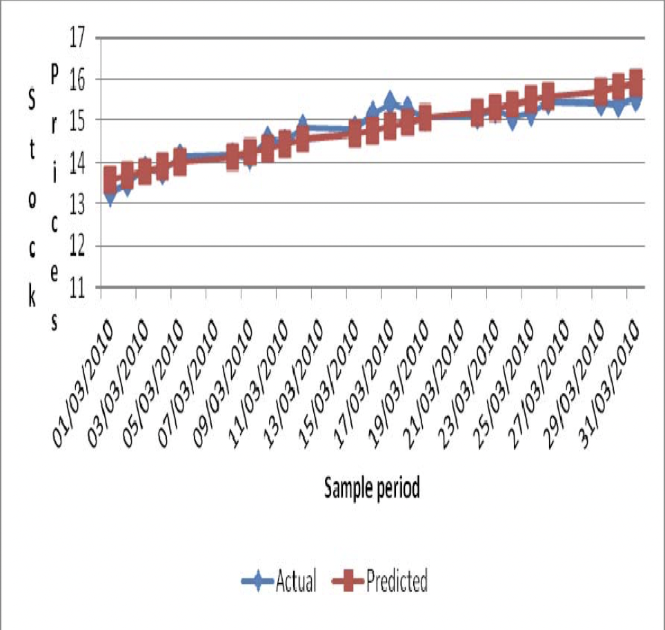
Figure 1. Actual vs Predicted stock price values of Nokia Stock Index [12]

Table 1. Metrics for NIFTY50 and top 4 indices [12]

The LightGBM and XGBoost models both focus on improving gradient boosting decision trees (GBDT). XGBoost was developed first by Chen and Guestrin as a scalable ML system for GBDT [13]. It is used in a wide variety of problems, ranging from classification to prediction [13]. The creators attribute this popularity to the system’s scalability, running over ten times faster than other solutions and scaling to billions of examples in memory-limited scenarios [13]. XGBoost introduces four main innovations to tree learning: an algorithm for handling sparse data, a justified weighted sketch for handling weights in tree learning, parallel computing for speed, and out of core computing to process billions of examples on a desktop [13]. Overall, XGBoost is still one of the best systems for GBDT.

However, Ke et al. improved current GBDT systems, such as XGBoost, focusing on their problems with efficiency and scalability that were still unsatisfactory for problems with high feature dimensions and large data sets [14]. The paper proposed two new improvements: Gradient-based One-Side Sampling (GOSS) and Exclusive Feature Bundling (EFB) [14]. GOSS’s principle is that data instances with larger gradients have a proportionally larger effect on the computation of information gain and contribute greater to it. Therefore, GOSS aims to keep larger gradients and only randomly drop smaller gradients, instead of randomly dropping all instances. This leads to a more accurate gain estimation with the same target sampling rate [14]. EFB works to reduce feature spaces, as there can be some features that are mutually exclusive in a large and sparse feature space. Ke et al. designed an algorithm to safely bundle these exclusive features, and called it EFB [14]. LightGBM can accelerate the training process by up to over 20 times while achieving almost the same accuracy [14]. One problem with LightGBM however is that it is very prone to overfitting with small datasets, and therefore the problem of using XGBoost or LightGBM depends on the situation.

In order to find out which system of GBDT was the best for stock prediction, Yang et al. ran an experiment with stock market data from Jane Street, to compare both models with a neural network and their own proposed model of a fusion of XGBoost and LightGBM in a 1:1 ratio [15]. They evaluated using a unity value, which is calculated with the following formula:

\( u=min(max(t,0),6)Σ{p_{i}} \) (2)

where

\( {p_{i }}=\sum _{j}^{0}(weigh{t_{ij}}*res{p_{ij}}*actio{n_{ij}}) \) (3)

and

\( t=\frac{Σ{p_{i}}}{\sqrt[]{Σ{{p_{i}}^{2}}}}\sqrt[]{\frac{250}{|i|}} \) (4)

when for each date i, each trade j will correspond to the following weight, resp, and action, and |i| is the total number of unique dates in the test dataset [15]. With the above evaluation method and four models created, they yielded Table 2 which describes the unity value [15]. Another study conducted by Ye et al. utilized the same methodology for Jane Street stock prediction and yielded a similar table with LightGBM outperforming XGBoost in the unity value [16].

Table 2. Utility score of the four models

The LSTM model is a variant of recurrent neural networks (RNN), and its main purpose is to solve the exploding/vanishing gradient problem. This allows it to process longer time series data without problems with its gradient. The LSTM adds a new state to hidden layers called the cell state and three new aspects for memory to a traditional RNN: an input gate, output gate and forget gate. The key addition is the cell state, which runs smoothly through each node with only a few linear interactions. This allows it to pass through information that is mostly unchanged, retaining older data values. The first interaction with the cell state is the forget gate, which decides what information to retain and forget after the previous layer finishes. Then, an input gate allows new information from the current node to pass through, which combines a sigmoid function to decide which information to update, and a tanh function to normalize the new values that are added to the state. Finally, to decide what to output, the hidden state separate to the cell state goes through a sigmoid function, choosing which values to carry on, and is then multiplied with a normalized cell state via the tanh function.

Another variant of the LSTM is the gated recurrent unit (GRU), which adds a reset and update gate. The reset gate controls how current and historical information is combined, and the update gate decides how much historic memory should be contained in each node. Sethia and Raut tested the viability in LSTMs and GRUs in stock prediction, comparing it to more traditional models such as support vector machines (SVM) and a simple feedforward network trained with backpropagation [17]. After running independent component analysis to choose features, they decided on 12 components for the final dataset. They used S&P 500 Open, High, Low, Volume and Adjusted Close information from the Yahoo Finance API as well as other technical indicators, mainly for volume, trend, momentum, and volatility [17]. Table 3 displays the results they achieved.

Table 3. Performance Comparison Between Models

Another notable study conducted on the viability of LSTMs in stock prediction was Bhandari et al. which searched for the optimal number of parameters for LSTMs [18]. They tested it on the S&P 500 index fund as well, arriving at the conclusion that single layer LSTM models with around 150 neurons have a better fit and accuracy than multilayer LSTM models [18].

3. Comparison, limitation and prospects

This paper covered four prevalent models in the stock market prediction scene, and showed the performance of each one, and some other models as well. Although each paper uses different metrics to evaluate their model, a prevalent theme can be seen that LSTMs and variants of it performed the best when compared to ARIMA and GBDT methods. ARIMAs are known to be robust and efficient, but are lacking in long-term prediction, only matching ANN methods in short-term predictions. XGBoost can’t handle categorical data, so it must be converted to numerical before being inputted. LightGBM doesn’t run into this problem, and is overall a good way to predict the stock market. However, LSTMs just perform better overall while sharing similar problems to LightGBM, making it a better choice. LSTMs perform better than LightGBMs because they can capture better nonlinear time-series data, which allows it to be more consistent and see better results than ARIMAs or decision trees. However, despite being the most optimal method for stock prediction out of the ones discussed in the paper, LSTMs are not perfect. As Sethia and Raut explained, LSTMs cannot predict extreme price dips or sharp price spikes, which might be caused by dramatic events in the economy such as an election or a war [17]. They also stated that the model could be made resistant to this if the input dataset includes economic factors like interest rate and GDP growth [17]. Another possible way to predict these sudden changes is by incorporating LSTMs with sentiment analysis, as many studies have done using twitter comments [18]. This could be effective as social media is gaining influence faster than ever, and could potentially affect the stock market. Another strategy that Gupta showed was to employ large language models (LLM) to analyse company financial data and predict which stocks to buy and sell [19]. This proved to have greater returns than the S&P 500 index fund. Other future improvements include a hybrid model which combines the models discussed above or with sentiment analysis.

4. Conclusion

To sum up, for the longest time, stock markets have challenged researchers and investors to try and predict it. With a myriad of methods at their disposal, keeping track of all of them is nearly impossible. This paper is not all-inclusive. Many innovations are being made to further optimize the current models and methodologies for investing in and predicting the stock market, such as creating hybrid models and trying to predict for long term investments. Some of the most efficient methods are kept confidential, as once introduced to the public they could become ineffective. Because of the constant development of the field and changing of current knowledge and available data, this paper doesn’t try to give a shallow explanation of all methods currently known, but instead explains four machine learning models that are currently most used in stock prediction, showing the results and methodologies of previous studies conducted, the potential downsides, and improvements that could be made that could be made to them and the field in general.

References

[1]. Abu-Mostafa Y and Atiya A 1996 Applied Intelligence vol 6(3) pp 205–213.
[2]. Zhong X and Enke D 2017 Expert Systems with Applications vol 67 pp 126–139.
[3]. Fama E 1970 The Journal of Finance vol 25(2) pp 383–417.
[4]. Chong E, Han C, and Park F C 2017 Expert Systems with Applications vol 83 pp 187–205.
[5]. Shah D, Isah H, and Zulkernine F 2019 International Journal of Financial Studies vol 7(2) p 26.
[6]. Velay M and Daniel F 2018 arXiv preprint arXiv:1808.00418.
[7]. Nesbitt K and Barrass 2004 IEEE Computer Graphics and Applications vol 24(5) pp 45–55.
[8]. Ballings M, Van den Poel D, Hespeels N, and Gryp R 2015 Expert Systems with Applications vol 42(20) pp 7046–7056.
[9]. Bollen J, Mao H, and Zeng X 2011 Journal of Computational Science vol 2(1) pp 1–8.
[10]. Seng J L and Yang H F 2017 Kybernetes vol 46(8) pp 1341–1365.
[11]. Ariyo A, Adewumi A, and Ayo C 2014 UKSim-AMSS 16th International Conference on Computer Modelling and Simulation p 137.
[12]. Devi B U, Sundar D and Alli P 2013 International Journal of Data Mining & Knowledge Management Process vol 3(1) pp 65–78.
[13]. Chen T and Guestrin C 2016 Proceedings of the 22nd acm sigkdd international conference on knowledge discovery and data mining pp 785-794.
[14]. Ke G, Meng Q, Finley T, et al. 2017 Advances in neural information processing systems vol 30.
[15]. Yang Y, Wu Y, Wang P, and Jiali X 2021 E3S Web of Conferences vol 275 p 01040.
[16]. Ye F, Wang J, Li Z, Jihan Z, and Yang C 2021 6th International Conference on Intelligent Computing and Signal Processing (ICSP) pp. 385-388.
[17]. Sethia A and Raut P 2018 Information and Communication Technology for Intelligent Systems pp 479–487.
[18]. Bhandari H, Rimal B, Pokhrel N, Rimal R, Dahal K, and Khatri R 2022 Machine Learning with Applications p 100320.
[19]. Tiwari T, Gururangan S, Guo C, et al. 2023 arXiv preprint arXiv:2306.03235.
Cite this article
Wu,N. (2024). Analysis of ARIMA, LightGBM, XGBoost, and LSTM models for stock prediction. Applied and Computational Engineering,54,76-81.
Data availability
The datasets used and/or analyzed during the current study will be available from the authors upon reasonable request.
Disclaimer/Publisher's Note
The statements, opinions and data contained in all publications are solely those of the individual author(s) and contributor(s) and not of EWA Publishing and/or the editor(s). EWA Publishing and/or the editor(s) disclaim responsibility for any injury to people or property resulting from any ideas, methods, instructions or products referred to in the content.
About volume
Volume title: Proceedings of the 4th International Conference on Signal Processing and Machine Learning
© 2024 by the author(s). Licensee EWA Publishing, Oxford, UK. This article is an open access article distributed under the terms and
conditions of the Creative Commons Attribution (CC BY) license. Authors who
publish this series agree to the following terms:
1. Authors retain copyright and grant the series right of first publication with the work simultaneously licensed under a Creative Commons
Attribution License that allows others to share the work with an acknowledgment of the work's authorship and initial publication in this
series.
2. Authors are able to enter into separate, additional contractual arrangements for the non-exclusive distribution of the series's published
version of the work (e.g., post it to an institutional repository or publish it in a book), with an acknowledgment of its initial
publication in this series.
3. Authors are permitted and encouraged to post their work online (e.g., in institutional repositories or on their website) prior to and
during the submission process, as it can lead to productive exchanges, as well as earlier and greater citation of published work (See
Open access policy for details).