1. Problem Definition

New York City Taxi and Limousine Commission (TLC) declares in their mission statement, "The mission of the Taxi and Limousine Commission is to ensure that New Yorkers and visitors to the City have access to taxicabs, car services, and commuter van services that are safe, efficient, suffciently plentiful, and provide a good passenger experience." However, 100,000 For Hire Vehicles and new Borough Taxi program (also known as the Street Hail Livery program) that has licensed thousands of green Borough Taxis to serve areas of New York not commonly served by yellow medallion cabs cannot resolve the issue with unmet trip demand. Unmet Trip Demand is a situation when New Yorkers or tourists would like to take a taxi, but hardly can do it and should spend more than 5 minutes to find one. It is usually happening in areas of New York City (NYC) historically underserved by the taxi industry. The major objective of this Capstone project is to identify the most underserved locations, explore contributing factors, and develop a model to predict demand in underserved areas across New York City. The client is Taxi and Limousine Commission, the agency responsible for licensing and regulating New York City’s medallion (yellow) taxicabs, for-hire vehicles (community-based liveries, black cars and luxury limousines), commuter vans, and paratransit vehicles ¹. The client is looking for reproducible and reasonably interpretable metrics that could help it identify unmet trip demand using existing taxi trips data.

2. Previous Work

Last year the capstone was done by another group of CUSP students. The approach was to tackle the problem from the observed demand and supply point of view meaning using the available taxi occupancy and vacancy data to predict unmet demand. The taxi data was broke down to Building Block Level (BBL) and per minute. Then the number of pick up and the number of vacant taxi per minute were calculated for each BBL. The ratio of the pickup to supply was defined as unmet demand. The method is not answering the question of defining unmet demand since it only gives the demand where a taxi is available but ignores the fact that there might be neighborhoods in NYC which have demand but no taxi supply hence that demand is not captured in their project.

3. Literature Review

Existing studies that analyzed similar questions to the project’s research agenda were driven by exploring of relationship between taxi supply and passenger trip demand all over the world. A study on the Asian market revealed spatio-temporal patterns to help taxi drivers spend less time for cruising [1]. Another example of demand prediction introduced based on city district scale in Munich, revealed timed-variant demand prediction for individual districts [2]. Mineta National Transit Consortium presented a report with results of taxi demand across time and space using GPS data from taxis [3].

Inspired by several studies that applied simulation methods in finding patterns, deriving formulas for the processes similar to the current project’s processes, and based on the characteristics of the data, the team developed a second approach by assuming the number of taxis records marked as free status in a given time interval in a given Census Tract follows a Poisson distribution. Sanghoon Lee’s book Communications in StatisticsSimulation and Computation identied a cyclic behavior in NHPP (Nonhomogeneous Poisson process) [4]. Later Larry Leemis introduced a way to estimate the mean λ(t) in NHPP using a linear function [5]. In the book Simulation published in 2013, Sheldon Ross further verified that using Poisson process with a time-dependent arriving rate function λ(t) was appropriate for studies associated with human activities [6].

The data points for this project are records of taxis with free status that satisfy the following two conditions:

1. The number of free status records in two disjoint time intervals are independent;

2. The probability of an occurrence of such taxi record during a small time interval is proportional to the entire length of the time interval.

Therefore, the free taxi records could be treated as Poisson random variables. A similar method was developed in a study "Where to wait for a taxi" which focused more on studying drivers behaviors through their driving patterns [7]. The focus of the project is more on the counts in each pointed area instead of the exact moving path the taxi drivers picked, the team use the time intervals and measure the level of availability to find areas being underserved. There is a possibility to use probabilities as outputs and unselect the parked vacant taxis when counting the free records, if necessary.

Poulsen et al [8] compared Green Taxi against Uber pickup data to locate the areas of NYC where TLC loses the greatest share of the market. The comparison was performed on the data collected between April and September of 2014. The authors performed the following data processing and analysis:

1. Merging Green Taxi and Uber data with zip code shapefiles through geoprocessing, grouping the pickup counts per zip code;

2. Splitting the data into sections of time periods: by week of year, by hour of the day, by weekday / weekend and by demographics;

3. Plotting choropleth map and search for significant differences.

The major findings of the article are as follows:

• Demand for Green cabs is still growing, but that the number of Uber rides in the same area is growing more rapidly.

• In relatively poor neighborhoods, Green cabs are performing better than Ubers.

• No differences between Green Taxi and Uber are found for weekdays/ weekends patterns.

Lu et al [9] applied several clustering techniques on the GPSdata of taxi pickups in order to differentiate the areas according to the demand. The data used in the research was collected in Shanghai from April, 1, 2015 to April, 30, 2015 by Shanghai Qiangsheng Intelligent Navigation Technology Company and contains GPS coordinates and time of individual taxis. The approach is as follows:

1. Extract pick-ups and drop-offs, calculate distributions.

2. Cluster different locations of the city by pick-up distributions.

3. Analyze clusters, determine hot-spots.

As a result of the research, the authors identify the hotspots of the city and introduce a new modification of the DBSCAN clustering algorithm that helped them to improve the performance of the DBSCAN by 10%.

Based on these above mentioned papers the team developed the third approach to compare Uber pickup with combined pick up data of Yellow and Green taxis.

Characteristics that distinguish areas such as population and employment have been used in studying demands. Ci Yang’s journal modeling Modeling taxi trip demand introduced a model that uses features including population and employment to predict the demand of taxis [3]. In Phase II, the team adapted this idea and selected similar features with several other relevant ones to build our models to estimate the unmet demand of yellow and green taxis.

As street topology could be a very important factor affecting drivers’ choice of roads, the team considers the street network in NYC in our study. Bin Jiang’s paper introduces an application of centrality measures based on graph principles and connectivity [10]. For an urban street network like the ones in NYC, these measures are able to capture its structural patterns and select the most important streets and intersections by evaluating the different roles of a street within the network in terms of connectivity, close-ness, and betweenness centralities. JonathanGross

In his paper Graph Theory and its Applications points out that streets of higher centralities tend to be more important, and they tend to attract more pedestrian flows in urban systems [11]. Therefore, the team believe that taxi drivers have the incentive to drive more often through the areas with roads that have better centrality to acquire more customers. On the other hand, areas with streets having lower centrality shall be less attractive to the taxi drivers and thus are more likely to have unmet demand.

The literature reviewed above and previous research studies help a lot to develop three major approaches in our two phases to identify unmet trip demand across NYC based on Census Tract properties, using combined data for Medallion, Street Hail Vehicles, and For-hire Vehicles (Uber) taxi services, and hunt for metrics that help Taxi and Limousine Commission update current policy and make taxis more accessible across NYC.

4. Data Description

In order to conduct the analysis, 10 different data set were used, including restricted Yellow and Green taxi trip records provided by TLC. The access to the data in restricted green and yellow environment that is provided through the CUSP compute remote desktop. To give a sense of the volume of the datasets, the largest one is the yellow and green taxicab dataset that is .5 TB and have over 4.5 billion of records in total.

Restricted data includes the following:

• Yellow taxicabs (TPEP) – trip records, breadcrumbs, rate4 and shift from two vendors i.e. VTS and CMT.

• Green taxicabs (LPEP) – trip records, breadcrumbs, rate4 and shift from two vendors i.e. VTS and CMT.

• For-hire vehicles (FHV) (various file formats)

The data acquired from open data sources covers the following fields:

• TLC data: www.nyc.gov

• Data of subway locations over the NYC: data.ny.gov/Transportation

• NYC Transit Subway Ridership data (2015): https://www.baruch.cuny.edu

• Tiger/Line street data – Road connectivity score (OSMnx package): https://www.census.gov/

• NYC crime data: catalog.data.gov/dataset

• American Community Survey(ACS) – demographic and socioeconomic information: www.census.gov/programs-surveys/acs

• Lion Street, Pluto & MapPluto Data – with land use data: www1.nyc.gov/site

• NYU Policy Map: the number of people working in the area

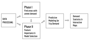
Figure 1. Methodology Workflow

5. Methodology Work-flow

5.1. Workflow

The flowchart in Figure 1 demonstrates the methodology workflow of our project.

The analysis section is divided into two phases. Phase I includes three approaches to filter selected census tracts. Based on those census tracts, using various related features, the team conducted random forest regression models.

Three approaches have been derived for the Phase I: using the counts of drop-offs as a proxy of demand to identify areas with potential unmet demand; evaluating the current rate of taxi supply to refine the results from the first approach from the supply side; using another proxy–Uber vs. street hail trends–to justify if the potential unmet demand is picked up by the increase of Uber services in some regions. Combining the results of all these three approaches validates the identified specific underserved census tracts with potential taxi unmet demand.

These three metrics uses three major datasets the Taxi Breadcrumb, Lion Street and the shapefile of Census Tracts. The study region covers Manhattan and other 4 boroughs; the counts are aggregated at different evaluation durations. The evaluation durations which come from the internal TLC study are taken into account the several important time ranges across NYC that impact taxi supply and passengers trip demand. Time ranges from Mondays through Saturdays include day rush hours (peaks) which are from 6am to 10am, middle day from 10am to 3.30pm, taxi shift change from 3.30pm to 4.30 pm, evening rush hours (peaks) from 4.30to 6pm, and 6-9pm,and night from 9pm to 6am. During the Sundays there are also several time ranges –12 to 2 am, 2 am to 2 pm, 2 to 4 pm, 4pm to 12am – that have been considered for this study. Note that the notation “weekdays” in the report and maps represents days from Mondays to Saturdays.

6. Phase I

6.1. Data Processing

6.1.1. MapReduce on taxi record counts

The yellow and green taxi breadcrumb data included geographic coordinates of all the taxis in every two minutes,

Table 1. Taxi Breadcrumb Data Format

Table 2. Data Processing Output from Hadoop

and if the taxi is vacant or occupied. The large volume of data was stored on a Hadoop Distributed File System, and pySpark was used to preprocess the data. Table 1 listed the column information in the breadcrumb data with an example:

The map and reduce jobs implemented for the three approaches in Phase I accomplished the following tasks:

• For pickups, a record is counted in the corresponding timeslot when a taxi’s passenger number increases from 0 to a number greater than 0.

• For dropoffs, a record is counted when a taxi’s passengers drops to 0.

• For vacant taxis, a record is counted when a taxi’s passenger number is 0.

After performing the mapping and reducing, the data format becomes the street IDs with the associated closest targeted counts in each evaluation duration for each of the tasks above. These intermediate products were then merged with the lion street dataset which included street IDs, and for each street the corresponding IDs of the Census Tracts on both sides of the street. Therefore, for each street ID, the corresponding targeted counts were added in both associated CTs. The output data contained the columns shown in Table 2.

6.1.2. Merge census tract and mapPLUTO Shapefile

By merging the reduced yellow and green taxi breadcrumb data with the mapPLUTO shapefile using Census Tract ID, the data were ready for further analysis.

6.2. Approach 1 Using Dropoffs to Proxy Demand

With lack of data on the demand side, and with the assumption that a person who takes a taxi to go back to a place are likely to request a taxi for a pickup when he leaves from there, the team found the number of taxi dropoffs in an area to be a good proxy of residents’ usage of taxis. Given an area, the large volume of dropoffs suggests the high demand of taxies associated with this area, and the much fewer pickups indicate that it is harder for people traveling from this place to get a taxi on the street, which is a reliable evidence of "unmet demand".

With such assumption, the first approach aimed to identify underserved areas by finding regions where the number of yellow & green cab pickups were significantly lower than that of drop offs. To avoid time lag issues, all comparisons were performed using aggregated dropoff and pickup counts for the whole month (January 2015 in our analysis).

The evaluation was based on the ratio of the number of pickups and dropoffs in each Census Tracts for each evaluation duration. The equation can be expressed as the following:

Pickup Counts < c × Dropoff Counts

As is shown, for a Census Tract reaching certain taxi trip numbers, the smaller the ratio c, the larger the discrepancy, and the more likely the area is being underserved.

As there were many places associated with small c ratios, the team found it reasonable to use 25% as the partition criterion among a range from 10% to 75% to label a desired number of "underserved" regions. Both ratios and the absolute difference in counts were taken into con-sideration to ensure the comparability of different Census Tracts. As is shown in Figure 2, the colors of map represent the different ratio intervals — except for the brown and black ones which represent areas with no pickup or drop-of information. For the all other regions, it can be observed that the darker the color, the similar the pickup and drop-of counts. The taxi pickups in red areas are more than 90% of drop-offs; in white areas the pickups only make up less than 25% of drop-offs.

By taking into account the taxi activities and the differences between drop-of and pickup counts, the team would never treat and 10/30 the same. For the study, the team used 86, which was the first quartile of all the differences between dropoff and pickup counts, as the threshold (Figure 3). If in a Census Tract the ratio C is small with substantial difference in counts, then it is more convincing that unmet demand occurs in that place. As the ratio map indicates that many outer boroughs have small differences in counts while these areas are in white in the difference map (Figure 2, 3), it is not applicable to draw any conclusion for these regions from this approach.

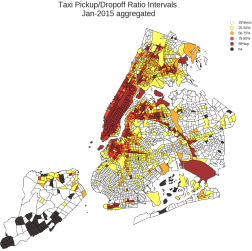
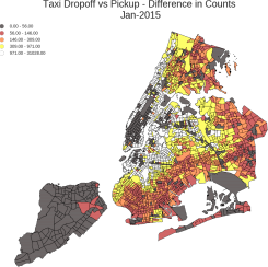
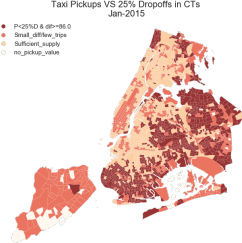
Figure 4. Taxi pickup counts versus 25% dropoff counts in NYC census tracts in January 2015.

Overlapping the ratio map (with 25% as the partition criteria) and the corresponding difference map (using counts 86 as the threshold), the team obtained the Census Tracts with potential unmet demand for each evaluation duration for days in January. Figure 4 is an output map example demonstrating the patterns. The areas in burgundy are CTs satisfying both conditions and that are the findings of this approach. Places such as the south west region of Brooklyn, north east Queens, and north Bronx are marked as regions with the highest likelihood to have “potential unmet demand”. The areas in white are regions with no pickup information, which mostly locate in Staten Island. The regions in red are either with too few trips or small difference between dropoff and pickups, and they are not being evaluated in this approach. Further steps will be taken to further examine and determine the regions with “unmet demand”.

6.3. Approach 2 Availability of Vacant Taxis

In approach 2, the assumption is that if there are many free taxis roaming in a CT, then there is no unmet demand. Based on this assumption, to validate and refine the underserved areas found in approach 1 from the supply side, the team evaluated the frequencies of vacant taxis passing through each CT for a given evaluation duration. These computation were performed on the breadcrumb data of

January 2015. Counts were divided on 11 batches showing the number of records with free status across NYC Census Tracts in each evaluation duration.

Based on the feature of the yellow/green cab breadcrumb data, each pin is recorded every 2 minutes; therefore, it is proper to assume that whenever a free taxi status is captured, the taxi has already been free for the past 2 minutes (under the optimal condition where everything is evenly distributed). This means that for each record of a free taxi status, it indicates an availability in that 2 minutes. The team treated each “free status” independently disregarding the associated taxi IDs, as if every record represented a different taxi, then the corresponding free minutes is equal to the record interval, and the total free minutes can be represented as follows:

Total Free Taxi Minutes = (FreeCountt × RecordIntervalt )

In the equation, T is the evaluation duration the team examined, and t is the moment of a pinned record within duration T. The record interval is a constant equal to 2 minutes. Therefore, the average free taxi availability rate is defined as the following formula:

Free Taxi Availability Rate = \( \frac{Total Taxi Free Minutes}{ \begin{array}{c} \\ Evaluation Duration \end{array} } \)

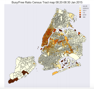
Figure 5. Ratio of Busy/Free taxis in NYC between 8:20am and 8:30am on Mondays to Saturdays in January 2015.

If the availability ratio is equal or more than 1, it means that there is always at least 1 vacant taxi available in every minute throughout the evaluation period in the census tract. Regions with unmet trip demands are expected to have low availability rates.

For exploration purposes, the team firstly drew the busy/free ratio Figure 5 to evaluate the relationship between free taxi and busy taxi so as to evaluate the possible unmet demand. The majority of Manhattan have higher busy/free ratios in each of the selected 10 minute time interval (eg: 08:20 08:30, 08:40 08:50, etc.) between 8am and 9:10am from Mondays through Saturdays. However, the ratio was not able to reflect the volume of vacant taxis of different regions for comparison, the team developed the "Average Free Taxi Availability" evaluation metric shown above to extract more insights.

The output for the approach 2 were maps showing the different levels of taxi availability rates across NYC. Noticing that areas with potential unmet demands are expected to associate with lower average taxi availability rates, the team were able to spot the locations with sufficient taxi supplies and also the places where unmet trip demand are likely to exist.

Figure 6 demonstrates the taxi availability rates that have similar patterns in all the evaluation durations for each CT. As is shown, regions in orange and cream such as midtown and downtown Manhattan are places where on average there are at least 1 vacant taxis available in every minute of the evaluation period. Areas in red and burgundy have fewer vacant taxi roaming so unmet trip demands are more likely to exist in these regions. These potentially underserved areas are consistent with those found in the approach 1.

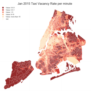
Figure 6. Average taxi availability rates across NYC in January 2015. This pattern preserves in all the evaluation durations.

6.4. Approach 3 Uber Pickups vs Yellow+Green

In Approach 3, the goal is to analyze and compare Uber pick ups with combined Yellow, Green and Uber pick ups for each census tract. The assumption is that if there were areas that have been underserved by Yellow and Green cabs, it has been addressed by Uber. Since Uber does not use the traditional street hailing but a sophisticated mobile app, it is more accessible by users.

The data of Uber pick ups of consecutive 6 months is available for period from April 2014 to September 2014. The data set contains pick up date-time, latitude and longitude of the pickup location. First using geo-processing the data set is merged with NYC Census Tract 2010 shapefile. After merging each pickup datapoint is assigned to a census tract. Then the data has been aggregated at a monthly level and time segments level as described in “identification of potential underserved regions” section for each census tract. This generated 6 data point (1 for each month) for each time segment at each census tract.

For Yellow and Green trip records, pre-processed breadcrumb data for year 2015 was used. This data set contains the following data for every 2 minutes for each vehicle: Vehicle ID, ping time, X-Y coordinates; occupancy/number of passengers, up to 3 nearest streets ID within 150ft of vehicle location. To make a comparison with available uber data, the team decided to use 6 consecutive months of data from April 2015 to September 2015. Because of the lack of availability of data, Uber data and breadcrumbs data was used fromt wo different years but the team tried to be consistent using the same months to capture any temporal patterns. To process the data spark filter was used to filter out data by aggregated by each month. After initial filtering, the occupancy column for two consecutive records with same vehicle ID was compared, if the occupancy changed from 0 to any other number, it was counted as a pick up and stored for further computation. After getting all the pick up record, the data was merged with lion census tract databased on the closest street ID on the breadcrumb data. Once merged record gets a right and a left census tract assigned to the pick up. Then the data was split for time segments as described in "Identification of potential underserved regions" section for each census tract and get the aggregated count. Sametime segment for each time segment count for all the 6 months are filtered out and put in one single file. This provided counts for pickup for each census tract for each time segment for every month from April to September, giving 6 data points for every census tract.

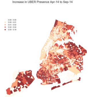
Figure 7. Percentage of increase in Uber Presence from Apr2014 to Sep-2014.The color scales are based on the the different level of uber/taxi growth ratios (i.e. 0.04 = 4% growth ratio).

Then the Uber pick-up count was added with Yellow+Green pick-up to get the total monthly pick-up for each CT and the ratio of Uber pick-up to total pick-up was calculated.

After calculating the ratio for each time segment a regression line is fitted on the 6 data points for each census tract. Whichever census tract saw a positive sloped regression line over the 6 months are considered to have their unmet demand fulfilled by Uber.

The final output of this analysis was a map (Figure 7) of all NYC and the list of CT with uber growth rate to show in all NYC census tract. Although uber pick up was significantly lower than combined yellow and green pick up, it was evident from the output that uber is catching up green taxicabs because it had a positive coeffcient for most of the CTs in outer boroughs.

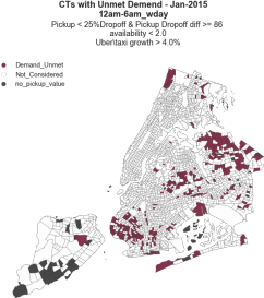
Figure 8. Map of NYC Census Tracts with unmet demands (burgundy areas) determined by the three approaches of phase I. According to the selected partition criteria, these regions have pickup counts less than 25% of dropoff counts, dropoff-pickup dispersion equal or greater than 86, uber/taxi growth ratio greater than 4%, and average availability rates less than 2/min between 12-6am on weekdays in January 2015.

6.5. Phase I Final Findings

After merging the output from the 3 approaches and the CTs that were common to all 3 approaches were identified as potentially underserved areas. There were 358 CT that were identified potential Unmet Demand, 33 of those CTs were identified with missing trip records and 1,787 CTs were identified with satisfactory Taxi Supply. Potentially Underserved Areas determined with all 3 Approaches were in Northeast Queens (Whitestone , Bayside, Flushing, Ridgewood) South Brooklyn (Bay Ridge, Bensonhurst, Coney Island, Brighton Beach), and North of the Bronx (Riverdale). (see Figure 8)

7. Phase II

Phase 2 of this study is based on the final findings from Phase 1. In this phase the goal is to compute the potential unmet for each Census Tract and to define taxi demand per underserved area in each defined evaluation period. Upon determining the CTs of interest, the Phase 2 aimed to address the following three questions. Firstly, finding out what are the most important features that have impact on the number of trips in NYC. Secondly, predicting the number of demanded trips for the under served areas. Finally, estimating the number of trips for areas where there is no pickup information.

The features which have been evaluated were selected based on the previous studies: population density, employment rate, median income, median rent, NYC Transit subway riderships, street network, office area, residential area, commercial area, retail area, and safety score. The Random Forest algorithm, which was able to capture the nonlinear relationships between the target variables(pickups) and the features, outperformed all the other machine learning methods being tested including KMeans clustering and Spatial Regression(linear regression), and it was selected for our predictive analysis.

7.1. Data Processing

Phase 2 used findings of phase 1 (number of pickups in the areas with suffcient number of pickups and under serves area)in 11 evaluation periods. In addition it used diferent data sets regarding the features used for modelling were: Office space, Retail space, Residential space, Commercial space, Income, Rent, Population, number of people working in the area, NYC Crime Data: Safety Score, Road connectivity score, Subway Ridership Count. Safety score dataset was available for intersection of streets that for this study by spatial join and getting the mean of the group of scores belong to a census tract this study ended up with a number for each census tract.

For the road connectivity feature, betweenness centrality, which evaluates how crucial a given street is as part of the shortest paths that connect any two other streets, was computed to analyze taxi pickups and unmet demand. The formula is shown as follows:

(gb,c denotes the set of all shortest or geodesic paths between band c.)

In this phase another feature was considered and evaluated was car ownership rate in the underserved area. The number of vehicle registration from Department of Transportation was processed to be used. But after initial data wrangling the team found out the data was available for only 160 zipcodes and it was not suffcient data to be applied at census tract level.

7.1.1. Feature Normalization

In order to get the best result , the features have been normalized by following formula:

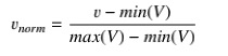
7.1.2. Outlier Removal

As the selected features could not capture the behaviour of the areas with exceptionally high pickups and dropoofs, e.g. transportation hubs and tourist areas, those areas were removed from the calculation. They accounted for 4% of all Census Tracts.

Evaluating the data for all the 11 evaluation periods showed the importance of the socioeconomic features on the number of pickups were almost the same. Therefore on this report only shows the outcomes of the evaluation duration between 12 am to 6am monday to saturday

Applying Random Forest feature importance method the feature importance was ranked as follows (See Table 3):

Table 3. Feature Importance Ranking

7.2. Predictive Model Section

To predict the number unmet demand trips in underserved areas including the areas with no available data, two different machine learning methods were applied : K-means clustering, and random forest regression. And random forest regression gave better prediction model. The findings shown on this report are the outcome of random forest regression model.

To build a prediction model the pick-up data was split in two parts: the areas with suffcient number of trips, and area with potential unmet demand. The model was developed using the 11 features as predictors and pick-up from CT with satisfactory as target variable. The generated regression model was then used to predict the required number of trip in the underserved areas. For the underserved areas with pickup values the unmet number of trips was simply calculated by subtracting the current number pf trips from the model generated predicted number of trips. For the underserved areas with no pickup values the model generated predicted number of trips are considered to be the number of unmet trips in those areas.

Using the model it was predicted that the total number of unmet trips in all 358 underserved CTs was 92 000 (or 12 trips per hour) trips per day.

For the evaluation period 12 am to 6am, the total number of trips in CTs with satisfactory supply, is approx. 300,000 and the total number of unmet demand trip in under served CTs is predicted to be approx. 12,000. Therefore in this evaluation period around 4% more trips are needed. Also the number of unmet trips in areas with no available pickup data is predicted to be approx. 1000.

7.3. Phase II Final Findings

Figure 9 shows the number of potential demanded trip in under served areas from 12am to 6 am. The areas in dark orange are ones with most unmet demand and the number of demanded trips are between 400800.

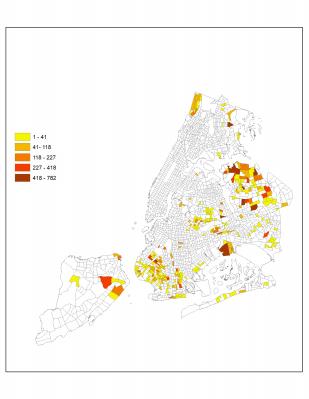
Figure 9. Unmet Trip Counts in Underserved Areas between 12am and 6am on Mondays through Saturdays in January 2015.

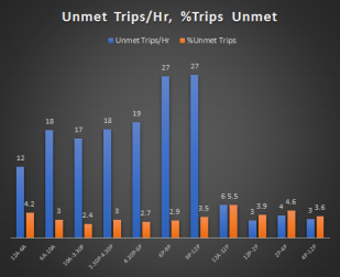
Figure 10. Bar plot of unmet trip counts and percentages per hour for each evaluation duration.

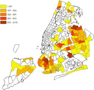
Figure 11. Map of Unmet Demand Prediction in NYC at Taxi Zone Level.

In the bar plot (Figure 10), the blue bars indicate the total number of predicted unmet demand per hour in the underserved CT for each evaluation period. The highest unmet demand was from 6pm to 12am with an average of 27 more trips needed per hour. Also the bars in red show the percentage of the trips that is needed to be increased in comparison to current number of trips. The highest percent is 6% that belongs to the evaluation period from 12am to 12pm on Sundays.

Figure 11 shows the underserved areas at Tax Zone level, that will be supplied to TLC to help make business decisions. The zones marked Dark red are the ones that predicted to have highest number of unmet demand. The number of unmet trips in these dark red areas are predicted to be between 1000 to 2000.

8. Case Study

As a showcase, one of the most underserved CT was picked to show the output from each computation stage. This ensus tract is located in Pomonok neighbourhood (Kew Gardens) in Queens (Figure 12).

The findings of the study indicates that this CTs has a pickup drop of the difference of 1645 which is much higher than the approach 1 threshold of 86, the ratio of pick-up and drop of is 4.6% which is much lower than the 25% threshold. The availability rate is 1.1taxi which is lower than the 2taxi/minute threshold. The Uber growth rate is 6.9% in this area which is slightly higher than the 4% cutoff rate, this can be another reason for this area has a very high demand because even Uber pickup had not grown so rapidly in this region therefore this indicates that the substitute services are not picking up on the unmet demand in this CT. Also, the evaluation period with highest demanded trips is 6pm to 9pm on weekdays. At that period around 550 more trips per hr are needed in this CT. On average, during the week this CT needs around 260 more trips per hr. But on Sundays the average number of demanded drops to 27 per hr. (See Figure 13)

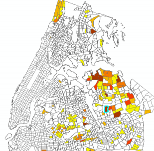
Figure 12. Case study location Pomonok neighbourhood Queens

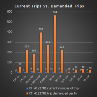
Figure 13. Trip Evaluation for Pomonok Neighbourhood in Queens.

9. Limitation

1. Lack of data

Due to no access to data on livery or black car companies, their trips or pick ups and their influence on the prediction model could not be analyzed. Also due to TLC’s strict data sharing policy, only limited data was obtained (e.g. six months of Uber trips and one year of Yellow and Green taxi data for year 2015)

2. Limited attributes

Data form Uber is limited by pickup locations only. Uber is not providing drop of locations that can be used to study in this project, so the current analysis on Uber’s influence in taxi market is based on pick ups locations. Other important features line drop of locations, price are not considered in this project.

3. Supply side

The metrics and methodologies are mostly from the “supply” side. Useful insights from the “demand” side such as passenger survey or real-time application that could collect their needs directly are not available.

4. Insuffcient features

It is apparent that there are some impacting facts that could be considered in a transportation project. However, features like Car ownership, Parking, Bus Routes, and Citi bike data could not be considered either due to unavailability or shortage of time.

5. Population density

The population density feature was considered as a whole for purpose of this project. The team understands that segregating this feature for different ages or genders groups could have meaningful impact on the model. For example, the CT with younger population might have more demand for taxi on a weekend night because of their participation in nightlife.

6. Street Network

The centrality scores assigned to each Census Tract were derived using the street network within that CT. The scores reflected the influence of a CT’s street topology to taxi pickups through taxi drivers preferences over different CTs. However, the method did not capture the characteristics of roads connecting the adjacent census tracts, which would also affect a driver’s decision on which CT to drive through next, especially when the taxi is vacant. A possible solution could be to assign a centrality score to each CT based on the entire road network including itself and its direct neighbors.

7. Spatial Autocorrelation

The Random Forest predictive model did not take into account the spatial autocorrelation that exists in the manhattan areas and outer boroughs. (See Figure 14).

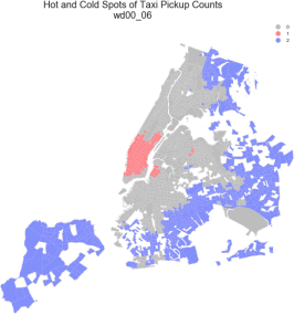
Figure 14. The heat map show the hot spots and cold spots of Taxi Pickup counts based on Moran’s I Statistics(Local). Autocorrelation occurs between the counts within a census tract and its neighbour tracts(neighbours are weighted) [12]. The cluster of red regions indicates that the tracts with high taxi pickup counts are likely to have adjacent tracts also having high number of pickups; the cluster of blue regions shows that the tracts with low number of pickups are more likely to have low counts in neighbour tracts.

10. Future Work

The team has successfully build a prediction model to predict unmet demand in underserved CTs in NYC. However the team expect these following suggestion can improve the model significantly:

1. To study unmet trip demand by using developed metrics and model, the whole year data of 2015 and 2016 from TLC could be used to conduct time series analysis, thus revealing seasonal patterns. With data from two different years a comparative stud-ies between them could have been done. This could contribute to the trend analysis to strengthen the existing metrics and models.

2. If data is available for more For-hire vehicles car services and companies such as Lift, WAV, liveries, etc., their influence in NYC taxicab industry across New York City could be studied

3. Public transportation network analysis can be considered to improve the current model and its predictive accuracy.

4. A new feature could be constructed in the predictive model to reflect the effect of SpatialAutocorrelation we found in the taxi pickups counts during the spatial analysis.

5. A real time application could be built to predict the number of needed taxi in a particular area or a particular time. This kind of application can make TLC aware of real-time taxi demand with visualization. With this application a dynamic heatmap can be plotted in the Carto, which will clearly shows the dynamic changes in taxi trip patterns (See Figure 15).

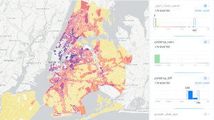
Figure 15. Carto Interactive Map and Real Time App

11. Conclusion

To summarize, the objective of this project was to reveal unmet trip demand, locate the most underserved areas, and build a prediction model. Unmet trip demand was defined by Taxi and Limousine Commission as a situation when person in NYC have to spend over five minutes to hail a taxi on the street. The project was splitted into 2 major phases to produce valid metrics and identify potentially underserved areas. Final results from Phase I, that aimed to analyze demand, supply, and substitutional services, revealed areas with unmet demand across New York City. These areas are North Bronx, East Queens, and South Brooklyn. The outcomes from the Phase II are the top 5 socio-economics features that mostly influence the trip demand and final prediction model that helps to predict trip demand. The features that mostly influence trip demand are o ce space, the number of people working in the area, residential space, income and rent. Prediction model for unmet trips resulted with 12,313 trips that needed at the underserved areas for specific time range from 12am to 6am. These results show that there is 4.2% shortage of taxi trips in the defined underserved areas out of the total number of trips across NYC. As a results of the project, we expect that TLC will be able to employ developed metrics and model to further trace the roots cause unmet trip demand in NYC and adjust current policies to meet passengers needs in taxi trips.

Author’s Contribution

Faculty Advisors: Dr. Huy T Vo., Dr. Kaan Ozbay

Project Sponsor: NYC Taxi and Limousine

All authors contributed equally to this work. Ziman Zhou, Pooneh Famili, Xin Tang, Anita Ahmed, Alexey Kalinin developed 3 different metrics to reveal potential unmet de-mand by using taxi data. Pooneh Famili and Ziman Zhou designed and implemented the prediction model. Alexey Kalinin and Anita Ahmed described the metrics and evaluated the model results. Xin Tang and Ziman Zhou created interactive map and demand statistics. All authors discussed the results, implications, future research, wrote and commented on the final report at all stages.

References

[1]. J.W. Powell, Y. Huang, F. Bastani, M. Ji, Towards Reducing Taxicab Cruising Time Using SpatioTemporal Profitability Maps., in SSTD (Springer, 2011), pp. 242–260
[2]. B. Jäger, M. Wittmann, M. Lienkamp, Journal of Tramc and Logistics Engineering Vol 4 (2016)
[3]. C. Yang, E. Gonzales, Transportation Research Record: Journal of the Transportation Research Board pp. 110–120 (2014)
[4]. S. Lee, J.R. Wilson, M.M. Crawford, Communications in Statistics-Simulation and Computation 20, 777 (1991)
[5]. L. Leemis, Estimating and simulating nonhomogeneous Poisson processes, in International Conference in Reliability and Survival Analysis (ICRSA), The University of South Carolina (2003)
[6]. S. Ross, in Simulation (Elsevier, 2013), pp. 111–134
[7]. X. Zheng,X. Liang, K. Xu, Where to wait for a taxi?, in Proceedings of the ACM SIGKDD International Workshop on Urban Computing (ACM, 2012), pp. 149–156
[8]. L.K. Poulsen,D. Dekkers, N. Wagenaar, W. Snijders, B. Lewinsky, R.R. Mukkamala, R. Vatrapu, Green Cabs vs. Uber in New York City, in Big Data (BigData Congress), 2016 IEEE International Congress on (IEEE, 2016), pp. 222–229
[9]. L. Zhang, C. Chen, Y. Wang, X. Guan, Exploiting Taxi Demand Hotspots Based on Vehicular Big Data Analytics, in Vehicular Technology Conference (VTC-Fall), 2016 IEEE 84th (IEEE, 2016), pp. 1–5
[10]. B. Jiang, C. Claramunt, GeoInformatica 8, 157 (2004)
[11]. J.L. Gross, J. Yellen, Graph theory and its applications, discrete mathematics and its application, series editor kh rosen (2005)
[12]. A. Getis, J.K. Ord, Spatial analysis: modelling in a GIS environment 374 (1996)
Cite this article
Ahmed,A.;Kalinin,A.;Famili,P.;Tang,X.;Zhou,Z. (2024). Predicting taxi unmet trip demand. Applied and Computational Engineering,47,287-305.
Data availability
The datasets used and/or analyzed during the current study will be available from the authors upon reasonable request.
Disclaimer/Publisher's Note
The statements, opinions and data contained in all publications are solely those of the individual author(s) and contributor(s) and not of EWA Publishing and/or the editor(s). EWA Publishing and/or the editor(s) disclaim responsibility for any injury to people or property resulting from any ideas, methods, instructions or products referred to in the content.
About volume
Volume title: Proceedings of the 4th International Conference on Signal Processing and Machine Learning
© 2024 by the author(s). Licensee EWA Publishing, Oxford, UK. This article is an open access article distributed under the terms and
conditions of the Creative Commons Attribution (CC BY) license. Authors who
publish this series agree to the following terms:
1. Authors retain copyright and grant the series right of first publication with the work simultaneously licensed under a Creative Commons
Attribution License that allows others to share the work with an acknowledgment of the work's authorship and initial publication in this
series.
2. Authors are able to enter into separate, additional contractual arrangements for the non-exclusive distribution of the series's published
version of the work (e.g., post it to an institutional repository or publish it in a book), with an acknowledgment of its initial
publication in this series.
3. Authors are permitted and encouraged to post their work online (e.g., in institutional repositories or on their website) prior to and
during the submission process, as it can lead to productive exchanges, as well as earlier and greater citation of published work (See
Open access policy for details).