1 Introduction

Multi-label learning, which assigns multiple labels to a single sample, is prevalent in various fields such as text [1, 2], image [3-5], video [6, 7], and bioinformatics [7]. Regarding the class imbalance problems, the accuracy of the classifier on minorities can be severely impaired by class imbalance. Nevertheless, accurate classification of minority classes is essential because minorities have more significant information. Existing methods to handle class imbalance are divided into two groups. One is called algorithm adaptation which makes the classifier skewed to the minority, the other is data preprocessing, including oversampling and undersampling. Compared with algorithm adaptation, sampling methods have a wider scope of application because they do not rely on the choice of the classifier [8-10].

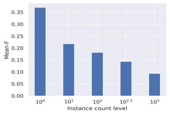
Figure 1. The impact of label imbalance on multi label classification

Figure 1 shows the evaluation results of Macro-F under different label imbalances in a multi-label dataset. This study found that the higher the imbalance level, the lower the value of Macro-F. Using neighborhood information has proven effective in multi-label contexts, particularly in oversampling strategies that mitigate overfitting and noise. This paper introduces a new sampling method that leverages label imbalance rates and neighborhood distribution. Comprehensive comparisons and parameter analyses of this method are presented in subsequent sections.

2 Related Work

2.1 Multi-label classification

Multi-label classification (MLC) assigns multiple labels to each instance within a dataset, Let \( D=\lbrace x_{i},Y_{i}|1≤i≤n\rbrace \) . For sample \( x_{i} \) , \( Y_{i} \) represents its associated labels as a binary sequence, where “ \( Y_{ij} \) =1” indicates presence and “ \( Y_{ij} \) =0” absence. The objective of MLC is to learn a function mapping \( x_{i}→Y_{i} \) for each instance.

MLC algorithms can be categorized by their utilization of label correlation: First-order methods like Binary Relevance (BR) [11] and Multi-label k nearest neighbors (MLkNN) [12] treat labels independently. Second-order approaches, exemplified by Calibrated Label Ranking (CLR) [13], account for pairwise label correlations. High-order methods, such as RAndom k-labELsets (RAkEL) and Classifier Chain (CC) [14-15], consider more complex label dependencies. While first-order methods offer simplicity, higher-order techniques provide a nuanced understanding of label relationships.

2.2 Measure imbalance

There are three different measures are proposed to estimate class imbalance between labels for multi-label data [16-18]. In Eq.(1), the Imbalance ratio per Label (IRLbl) is proposed to be calculated by mining the relationships between the labels.

\( IRLbl=c_{max}^{1}/c_{j}^{1} ( j∈1,2,3.....q ) \) (1)

As can be seen in Eq.(2), MeanIR is obtained by averaging the IRLbl about all labels. This study defines that a label with IRLbl >MeanIR is the minority label but IRLbl

\( MeanIR=\frac{1}{q}\sum_{j=1}^{q}IRLbl_{j} \) (2)

The coefficient of variation of IRLbl (CVIR) is a measure that quantifies the variation of IRLbl, reflecting the similarity of the degree of class imbalance across all labels.

\( CVIR=\frac{1}{MeanIR}\sqrt[]{\sum_{j=1}^{q}\frac{(IRLbl_{j}-MeanIR)^{2}}{1-q} } \) (3)

the high CVIR indicates that there are significant differences in the level of imbalance among the labels, while a low value indicates that the labels experience similar levels of imbalance.

3 Proposed method

MLSIN first calculates a matrix \( C∈R ^{n*n} \) that stores the proportion of majority class values in the distribution of sample neighborhood labels, this matrix records the proportion of k nearest neighbors of each sample that are not equal to their labels, where k is a hyper-parameters [19]. The calculation method is to first find the k nearest neighbor samples of each sample \( x_{i} \) , for each label \( l_{j} \) , and then calculate the proportion of kNN of sample \( x_{i} \) that are not equal to their labels. The calculation method is as shown in Eq.(4):

\( C_{ij}=\frac{1}{k}\sum_{x_{i}∈kNN_{x_{i}}}⟦Y_{ij}≠Y_{kj}⟧ \) (4)

where the notation \( ⟦Θ⟧ \) represents the indicator function, which yields 1 if \( ⟦Θ⟧ \) is true and 0 otherwise.

Next, MLSIN calculate the sample weight \( w_{i} \) for each sample in the dataset. The larger the sample weight, the easier it is to selected as the base sample during the sampling process. The specific steps of calculation are to calculate the values of the training sample \( x_{i} \) in matrix \( C \) . The specific steps of calculation are to sum the values of the training \( x_{i} \) in matrix C to obtain the weight \( w_{i} \) of a single sample, which can represent the difficulty of correctly predicting the minority labels associated with the sample. To simplify the formula, assuming the minority class value in the label is 1, the calculation formula is shown in Eq.(5):

\( w_{i}=\sum_{i=1}^{q}C_{ij}⟦Y_{ij}=1⟧ \) (5)

The sample type matrix T divides minority class samples into four categories based on their \( C_{ij} \) values, including intra-class (IC), boundary (BD), out of class (OB), and outlier (OT).

IC: \( 0 \lt C_{ij} \lt 0.3 \) , the intra class samples are located in areas with dense minority class samples.

BD: \( 0.3≤C_{ij} \lt 0.5 \) , boundary samples are located at the decision boundary, usually between minority and majority classes.

OB: \( 0.5≤C_{ij} \lt 0.7 \) , outliers are closer to the majority class than boundary samples. At the sample outside the boundary. When selected for generating new samples, the label values of the new samples will be directly set to minority classes.

OT: \( 0.7≤C_{ij} \lt 1 \) , outliers are surrounded by majority class samples.

In addition, the type of majority class samples is defined as majority (MJ). Let T={IC, BD, OB, OT, MJ} be the matrix that stores the distribution of neighborhood labels, and \( T_{ij} \) be the type value of \( Y_{ij} \) . After determining the sample type matrix T, the algorithm will make a correction to the sample type. For all OB samples, if one of its k nearest neighbor samples is of type IC or BD, the type of that sample will be corrected to BD.

The MLSIN algorithm presented in this text is a synthetic sampling method developed from the MLSOL algorithm. It takes into account both the label imbalance rate and neighborhood distribution. The pseudocode shown in Table 1 outlines the algorithm's process. Initially, it calculates the label imbalance rate and the imbalance weight as well as a matrix C representing the proportion of majority class values in the neighborhood label distribution. These variables are used to compute the sample neighborhood weight and type matrix T, which will be utilized for selecting base samples and generating new ones. The algorithm then iteratively selects a base and auxiliary sample for the generation of new instances and adds them to the dataset. The process concludes when the number of generated samples reaches a predetermined threshold, ending the oversampling method.

Table 1. Pseudocode of MLSIN

4 Experiments and Analysis

This study selected 12 MLDs that are widely used in different fields such as text, image, and bioinformatics, all data sets will be downloaded in MULAN. A simple feature selection approach is applied that retains the top 20% (Corel5k), top 10% (BibTex, medical, Enron) and the top 1% (rcv1subset), method is compared with two heuristic neighbor-based sampling methods (MLSMOTE, MLSOL) and two random sampling methods (MLROS, MLRUS), Especially, this experiment analyzed three label sets assigned methods (Union, Ranking, Intersection) about MLSMOTE [20, 21]. The sampling ratio p is selected from {0.01, 0.05, 0.1, 0.2, 0.3, 0.5, 0.7} for parametric sampling methods (MLROS, MLSOL, and MLRUS). What’s more, four standard multi-label learning algorithms (MLkNN, BR, CC, RAkEL) are used to display the universality of our methods. Regarding the BR, CC, and RAkEL, Decision-Tree is also used as the based classifier. Based on a rule-of-thumb, k=10 as the neighbor is set for MLkNN, k=3 and n=2q for RAkEL, and k=5 as the neighbor for MLSMOTE.

This paper chooses the multi-label evaluation metrics including Macro-averaged AUCROC (area under the receiver operating characteristic curve) to evaluate the performance of previous methods and the method proposed. Then, 5*2 cross-validation will be applied. Finally, to maintain the sample distribution of MLD, multi-label iterative stratification is applied to divide MLD into the training set and the test set.

The summary provided indicates that the MLSIN method outperforms other methods in AUC, showcasing significant improvement (Table 2). It tops average rankings across classifiers, suggesting wide applicability. Neighbor-based methods like MLSOL and MLSMOTE with Ranking also do well, but not as much as MLSIN. Conversely, MLRUS, due to its random undersampling nature, may eliminate crucial samples, making it less effective. The performance of MLSIN with MLkNN as a base classifier is noteworthy, and it is most effective in addressing imbalance within labels, essential for precision and recall in classification. However, in algorithms like RAkEL and CC, which consider label correlation, MLSIN's impact is less pronounced compared to MLkNN.

5 Conclusion

In the experiments, different settings for one parameter are used, while keeping others unchanged at the setting. The application of MLSIN improves the performance of the classifier. that proves to generate some samples will aid classifier learning from the training set. However, as the sampling ratio continues to increase, the performance of the classifier will decrease, because excess samples may distort the original class distributions, and then add to the difficulty of classification. In particular, for the base classifier RAkEL, which transforms the label subsets into classes. When the sampling ratio exceeds 0.1, the evaluation measures decrease significantly, mainly because RAkEL is sensitive to the change in the label set of samples. Otherwise, MLkNN is the best-performing classifier, and under different sampling ratios, the three evaluation measures perform relatively stable without significant decline. MLSIN obtains information from natural neighbors to generate samples, which can provide more guidance for neighbor-based MLkNN.

Research on existing multi-label resampling methods for handling imbalances reveals that current approaches often overlook the variations in label imbalance rates. Therefore, by integrating label imbalance rates with neighborhood distribution for sample selection, the sampling intensity for labels with a higher degree of imbalance is increased, allowing them to have a greater probability of being chosen during sample selection. A penalty strategy is introduced when classifying types of minority label samples, allowing for more cautious type correction and enhancing the information of minority class samples on the decision boundary. These methods effectively reduce the degree of imbalance in multi-label datasets, while also enhancing the classifier’s ability to learn from and classify minority class labels and decision boundaries, thereby improving classification performance.

References

[1]. G. Tsoumakas, I. Katakis, I. Vlahavas, Mining Multi-label Data [C]// Data Mining and Knowledge Discovery Handbook, 2009: 667-685.
[2]. Zhang M. L., Zhou Z. H. A review on multi-label learning algorithms [J]. IEEE transactions on knowledge and data engineering, 2013, 26(8): 1819-1837.
[3]. Tsoumakas G., Katakis I. Multi-label classification: An overview [J]. International Journal of Data Warehousing and Mining (IJDWM), 2007, 3(3): 1-13..
[4]. Buczak A. L., Guven E. A Survey of Data Mining and Machine Learning Methods for Cyber Security Intrusion Detection [J]. IEEE Communications Surveys & Tutorials, 2015, 18(2): 1153-1176.
[5]. Zhou F., Huang S., Xing Y. Deep semantic dictionary learning for multi-label image classification [C] Proceedings of the AAAI Conference on Artificial Intelligence. 2021, 35(4): 3572-3580.
[6]. Harding S. M., Benci J. L., Irianto J., et al. Mitotic progression following DNA damage enables pattern recognition within micronuclei [J]. Nature, 2017, 548(7668): 466-470.
[7]. Zhu X., Li J., Ren J., et al. Dynamic ensemble learning for multi-label classification [J]. Information Sciences, 2023, 623: 94-111.
[8]. B. Wu, E.H. Zhong, A. Horner, Q. Yang, Music emotion recognition by multi-label multi-layer multi-instance multi-view learning [C]// Proceedings of the 22nd ACM International Conference on Multimedia ACM, 2014: 117-126.
[9]. Rastogi R., Kumar S. Discriminatory label-specific weights for multi-label learning with missing labels [J]. Neural Processing Letters, 2023, 55(2): 1397-1431.
[10]. Chen Ming-Syan, Han Jiawei, Yu P.S. Data mining: An Overview from a Database Perspective [J]. IEEE Transactions on Knowledge and Data Engineering, 1996, 8(6): 866-883.
[11]. M.R. Boutell, J. Luo, X. Shen, C.M. Brown, Learning multi-label scene classification [J]. Pattern Recognition, 2004, 37(9): 1757-1771.
[12]. Zhang M. L., Li Y. K., Yang H, et al. Towards class-imbalance aware multi-label learning [J]. IEEE Transactions on Cybernetics, 2020, 52(6): 4459-4471.
[13]. Tarekegn A. N., Giacobini M., Michalak K. A review of methods for imbalanced multi-label classification [J]. Pattern Recognition, 2021, 118: 107965.
[14]. Mollas I., Chrysopoulou Z., Karlos S., et al. ETHOS: a multi-label hate speech detection dataset [J]. Complex & Intelligent Systems, 2022, 8(6): 4663-4678.
[15]. Charte F., Rivera A. J., del Jesus M. J., et al. Addressing imbalance in multilabel classification: Measures and random resampling algorithms [J]. Neurocomputing, 2015, 163: 3-16.
[16]. Charte F., Rivera A. J., del Jesus M. J., et al. MLSMOTE: Approaching imbalanced multilabel learning through synthetic instance generation [J]. Knowledge-Based Systems, 2015, 89: 385-397.
[17]. Chawla N. V., Bowyer K. W., Hall L. O., et al. SMOTE: synthetic minority over-sampling technique [J]. Journal of artificial intelligence research, 2002, 16: 321-357.
[18]. Pereira R. M., Costa Y. M. G., Silla Jr C. N. MLTL: A multi-label approach for the Tomek Link undersampling algorithm [J]. Neurocomputing, 2020, 383: 95-105.
[19]. Charte F., Rivera A., del Jesus M. J., et al. Resampling multilabel datasets by decoupling highly imbalanced labels [C]// Hybrid Artificial Intelligent Systems: 10th International Conference, HAIS 2015, Bilbao, Spain, June 22-24, 2015, Proceedings 10. Springer International Publishing, 2015: 489-501.
[20]. Liu B., Blekas K., Tsoumakas G. Multi-label sampling based on local label imbalance [J]. Pattern Recognition, 2022, 122: 108294.
[21]. [1] Zhang K., Mao Z., Cao P., et al. Label correlation guided borderline oversampling for imbalanced multi-label data learning [J]. Knowledge-Based Systems, 2023, 279: 110938.
Cite this article
Zhang,Z. (2024). Multi-Label Sampling based on Label Imbalance Rate and Neighborhood Distribution. Applied and Computational Engineering,57,104-111.
Data availability
The datasets used and/or analyzed during the current study will be available from the authors upon reasonable request.
Disclaimer/Publisher's Note
The statements, opinions and data contained in all publications are solely those of the individual author(s) and contributor(s) and not of EWA Publishing and/or the editor(s). EWA Publishing and/or the editor(s) disclaim responsibility for any injury to people or property resulting from any ideas, methods, instructions or products referred to in the content.
About volume
Volume title: Proceedings of the 6th International Conference on Computing and Data Science
© 2024 by the author(s). Licensee EWA Publishing, Oxford, UK. This article is an open access article distributed under the terms and
conditions of the Creative Commons Attribution (CC BY) license. Authors who
publish this series agree to the following terms:
1. Authors retain copyright and grant the series right of first publication with the work simultaneously licensed under a Creative Commons
Attribution License that allows others to share the work with an acknowledgment of the work's authorship and initial publication in this
series.
2. Authors are able to enter into separate, additional contractual arrangements for the non-exclusive distribution of the series's published
version of the work (e.g., post it to an institutional repository or publish it in a book), with an acknowledgment of its initial
publication in this series.
3. Authors are permitted and encouraged to post their work online (e.g., in institutional repositories or on their website) prior to and
during the submission process, as it can lead to productive exchanges, as well as earlier and greater citation of published work (See
Open access policy for details).