1. Introduction

The use of machine tools such as Computer Numerical Control (CNC) to process materials plays a vital role in the modern manufacturing industry[5].; the condition of various aspects of the machine dramatically determines the quality of the machined product . The condition test of the machine is the key to ensuring product quality and extending the machine's life. It is essential to monitor their status and provide an appropriate assessment. Due to the limitations of cost, available space and conversion principles, only a few physical variables, such as acceleration, force, displacement, acoustic radiation, temperature and flow conditions, can usually be measured. It is critical to transfer These data efficiently and extract useful information for monitoring machine status by statistical means or extracting functional signatures [7]. However, measurement instruments using Traditional methods are numerous and complex. In contrast, measurement and analysis systems

Virtual instrumentation technology collects the necessary data from sensors and data acquisition cards to meet the needs of test analysis. Virtual instrumentation consists of computer hardware resources, modularization hardware and software systems used for data analysis, communication, and operation interface. Systems based on Virtual Instruments LabVIEW have greater versatility, flexibility, compatibility and repeatability [1].

Sun et al. [7] developed the system using Arduino, Bluetooth and LabVIEW and used it to monitor the operation of a 5-axis CNC milling machine. An et al.[1] propose a Labview-based system that is applied to developing and testing CNC milling machines with an open architecture and extended to other machines and processes. Milfelner et al. [4] select cutting parameters and measure cutting forces as applications to present a systematic approach to designing a condition monitoring system for machine tools and machining operations.

Yeh et al. [8] developed a system to suppress cutting vibrations and control cutting torque and verified the feasibility of the design through experiments. The LabVIEW-based data collection systems and methods for data processing and analysis in these researches are exemplary attempts.

The purpose of this project is to collect data from the machining process of the CNC and process the data. The main objectives of the project are:

a) Write a LabVIEW software program.

b) Using the supplied hardware(myRIO) and the LabVIEW program to record data from CNC machine programs.

c) Processing data with MATLAB software.

d) Analysis and discussion of data.

There will be 4 parts in this report. It will

begin with an introduction to the background of the project and a review of the literature. Then, describe the steps and methods used in the project. Then, describe the experiments and the methods used for the project. The following section will show and discuss the processed data graphs. After discussing the recommendations for future research, the report will conclude with a summary of the study.

2. Experimental methodology

The purpose of the experiment is to use Labview to record the cutting force and torque of the industrial CNC machine tool in the milling process and to use Matlab for data processing. In the whole process, the CNC machine tool works at different spindle speeds and feed rates to process 9 holes. During processing, the thrust and torque parameter fluctuations of the drill bit are transmitted to the myRIO based on the 10,000 Hz sampling rate through the dynamometer and charge amplifier for recording. The experimenter needs to write and execute an FPGA program to complete the recording of these parameters.

3. Materials

The main equipment of the experiment is a Haas VF-2SS CNC machine in Figure 1. The processed mould is a square carbon steel. Kistler's dynamometer (The measuring range: +/-100nm and +/-10000n) and charge amplifier (voltage output: +/-10V) is shown in Figure 2. Figure 3 is a myRIO toolkit. Experimenters can use the components to design a program based on Labview and verify the operation of the program before the experiment.

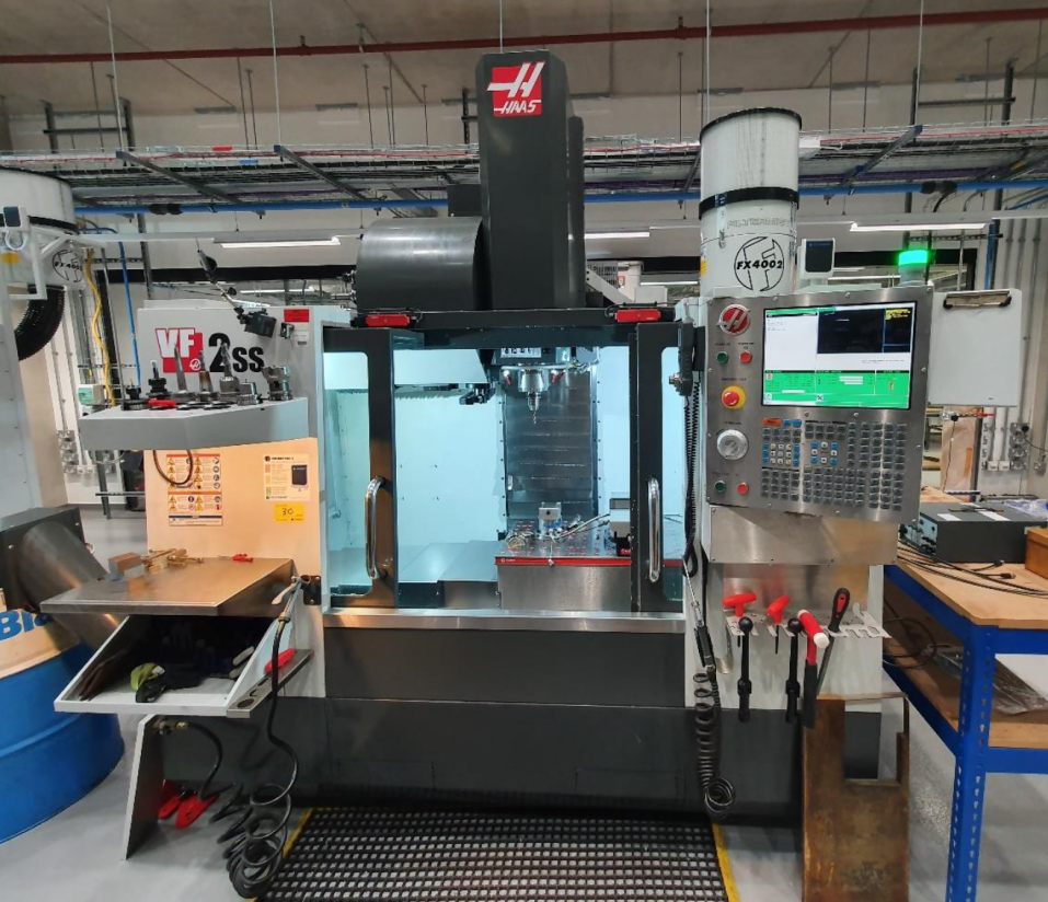
Figure 1. Haas VF-2SS CNC machine.

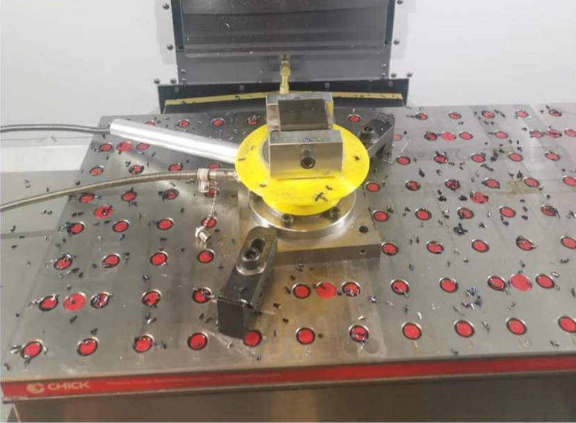
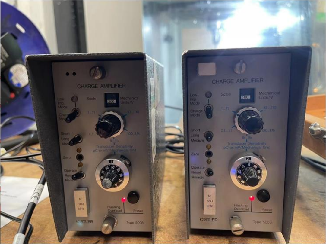
Figure 2. Kistler's dynamometer with mould (left) and charge amplifier (right).

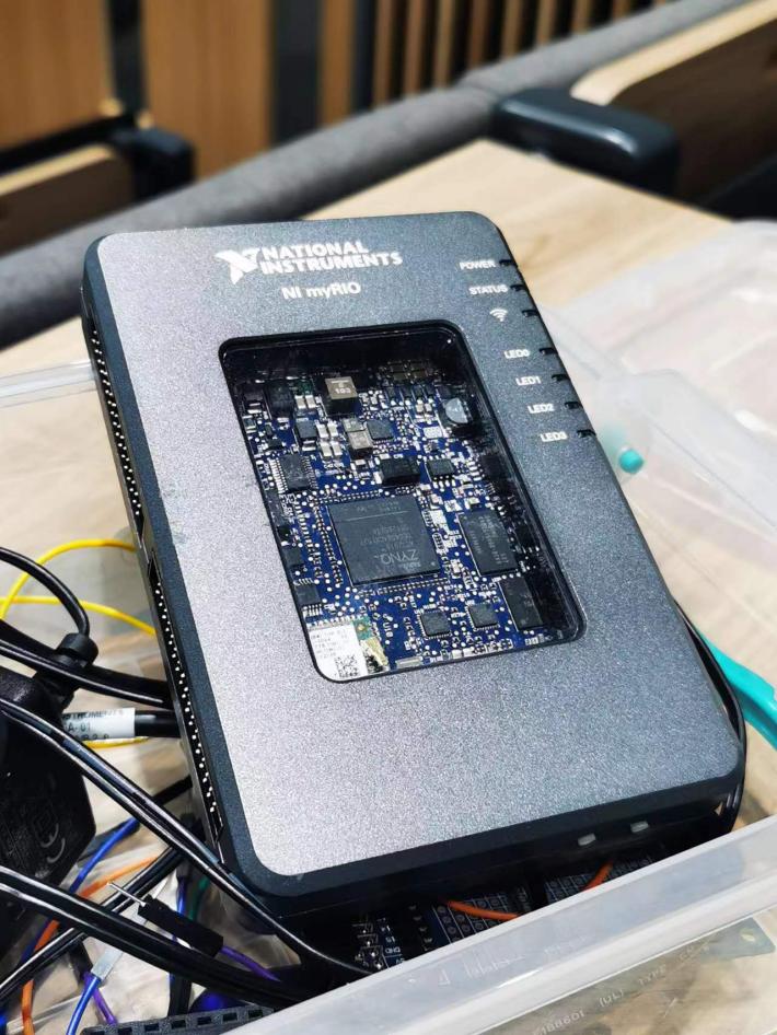
Figure 3. A myRIO 1900 toolkit.

In addition, a connector has been developed to transfer torque to channel A/AI0 of myRIO and thrust to channel A/AI1. A CNC machining program has been completed to facilitate the implementation of the 9 machining experiments in Table 1.

Table 1. CNC experiment parameter.

3.1. LabVIEW programming

There are three types of rotation speed and feed rate, so there are nine total combinations of the process. Therefore, the myRIO device will record the data of nine holes in the experiment.

This project uses the LabVIEW myRIO toolkit to write the DAQ programs. Since it is required to record the output of the CNC machine at a frequency of 10,000 Hz, the program must record

and store data at a very high speed. Therefore, in this experiment, FPGA will be utilized for data acquisition. The program will be divided into two parts: the host and FPGA. In addition, to cooperate with high-speed data acquisition, the TDMS method, which is more efficient than the CSV file, is used to record the data in the program.

The C port on the myRIO device is used in this project to connect to the CNC machine and receive data from the machine.

During the recording process, the program and the CNC machine started running simultaneously, and the data acquisition of the nine holes was completed automatically. After the CNC machine completed the process, the Labview program was also manually stopped. After that, the data of the CNC machine will be saved in a .tdms file generated in the host for subsequent data processing.

In the FPGA program, two FPGA I/Os are first created to receive the signals of the C port channel AI0 and AI1, respectively.

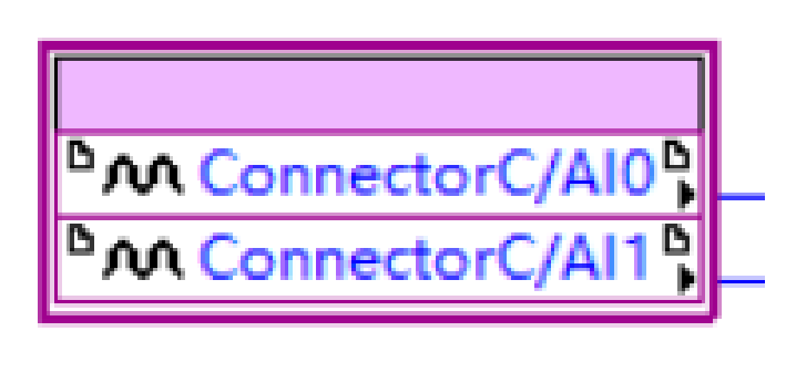
Figure 4. FPGA I/O.

Then a for loop was created to receive and create a single data point in a loop. In this vi, the loop timer is used to control the sampling frequency of the program, and a control is created to input the required frequency. It should be noted that uSec is entered in control instead of Hz.

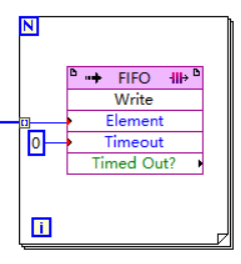
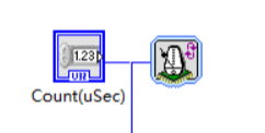
Figure 5. Loop and timer.

Finally, the front panel is shown in the figure, including the control of the input frequency and the waveform diagram of the display input signal.

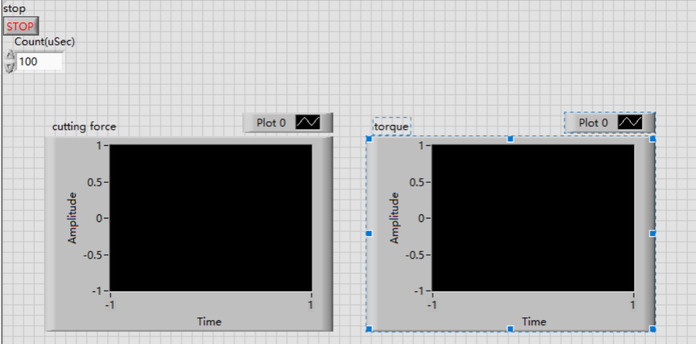
Figure 6. Diagram.

In the host program, we wrote a program to call vi in the aforementioned FPGA and save the data. In order to be able to save data at a high speed and accurately, the TDMS format is used in this program, and the operation is completed through the structure shown in the figure below.

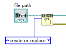
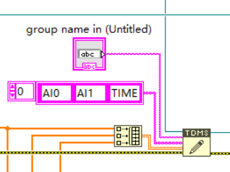
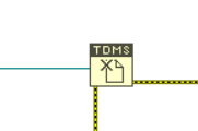
Figure 7. VI of TDMS format.

The final program is shown in the figure below:

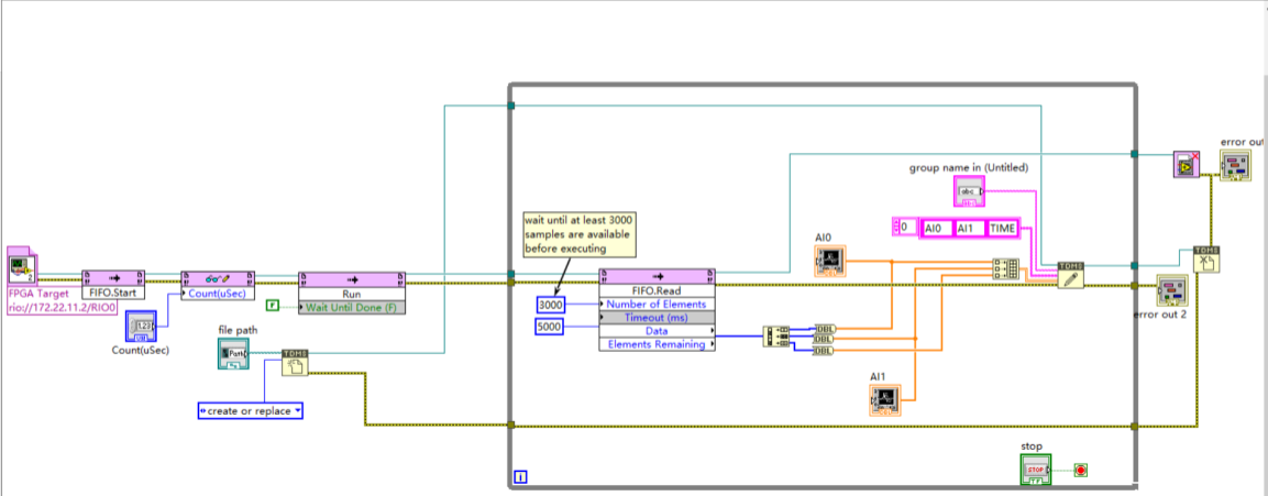
Figure 8. LabVIEW program.

3.2. MATLAB post-processing

The data after FPGA program execution is transferred from myRIO to a personal computer and stored as an Excel file. MATLAB program is the main tool for data processing. The MATLAB program created in this project can automatically complete data import, data processing and graph generation. This section introduces the main content and principles of MATLAB programming of this project.

3.2.1. Processing raw data. The analogy signal during the experiment is converted into a digital signal. Therefore, the raw data needs to be converted into corresponding force and torque values. The NI myRIO-1900 User Guide and Specification indicates that the formula for converting raw data values into voltage is

V = Raw Data Value × LSB Weight.

For AI and AO channels on the MSP connectors

\( LSB Weight = \frac{Nominal Range}{{2^{ADC Resolutio}}} = \frac{20}{{2^{12}}} . \)

The formula for calculating force (F, N) and torque (T, N*M) obtained by applying the calibration scale of the charge amplifier in Figure 2 is

F = V × calibration scale = Raw Data Value × \( \frac{20}{{2^{12}}} \) × 500

T = V × calibration scale = Raw Data Value × \( \frac{20}{{2^{12}}} \) ÷ 100 × 200

In addition, it is worth noting that the obtained original data may have an offset, and the offset should be removed before converting the value.

3.2.2. Split waveform data. In order for the split force and torque graphs to correspond to each other, select the same data interval for both. In the nodes of Figure 9, node-b is the starting point, and node-e is the ending point.

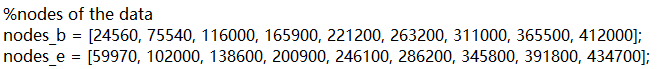
Figure 9. MATLAB code: Split data.

3.2.3. Remove noise. This project uses a MATLAB built-in command 'smoothdata' to remove noise. This method can process data more quickly than the three-point filtering method, and the resulting denoising effect is better. Since the original data has some extremely abnormal values (shown in the result section), the 'smoothdata' based on 'movmedian' is used for processing, because in this case the moving median can get more accurate results than the moving average.

3.2.4. Generate frequency spectrum. The code of the spectrogram of force and torque refers to the fast Fourier transform chapter of the official tutorial of MATLAB[1]. The signal parameters are set based on a sampling rate of 10000 Hz.

3.2.5. Other data processing. This project created a Function to calculate the mean value and standard deviation, and established 4 sets of curve fits based on the obtained data.

4. Result and discussion

This experiment collected a lot of data in about 48 seconds. Analysis is based on the collected data through the transformation of experimental data units, waveform analysis, noise analysis and noise elimination. Then, the experimental data were further analysed by establishing frequency graph and curve fit.

4.1. Processing raw data of thrust

By using MATLAB to convert the collected data from voltage to thrust and torque, then raw data are used to drew diagram below to show with the increasing of time, how thrust and torque are changed.

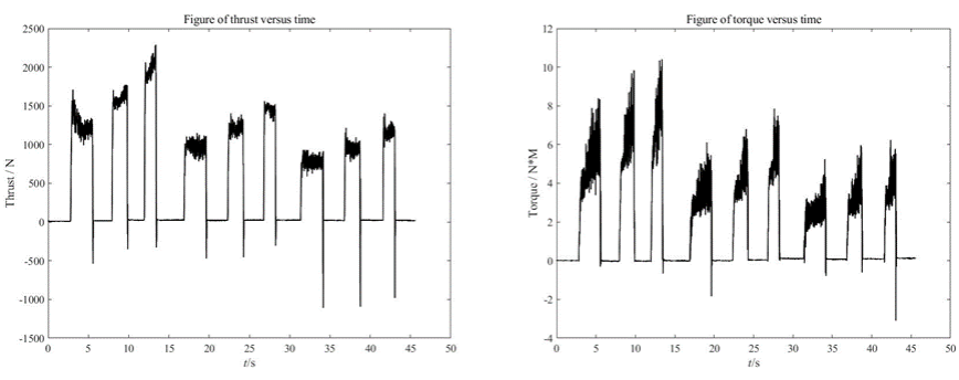
Figure 10. Processed row data of thrust and torque.

Figure 10 shows the peak value of 9 holes drilled by a CNC machine at different speeds and feed rates. On the left-hand side, it is thrust verses time, and on right hand side is torque versus time. Under the condition of high speed and high feed, the maximum thrust produced is about 2000N; the maximum torque is around 10N*M.

It can be clearly seen from the figure that if the speed is the same, the greater the feed, the greater the thrust, and the less time it takes (thinner column) to drill a hole. Torque has an increase tendency in value as it drills deeper.

Similarly, this figure also shows the relationship between the maximum peak value and drilling time of nine groups of drilling experiments.

4.2. Split waveform data of thrust and torque

By means of data slices, we magnify the time corresponding to the peak value of each group of forces, and obtain the following nine groups of data tables for thrust and torque respectively:

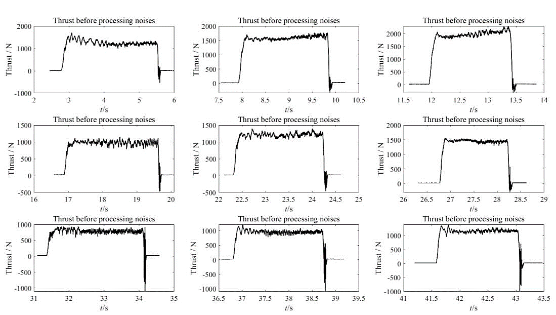
Figure 11. 9 sets of thrust data before processing noises

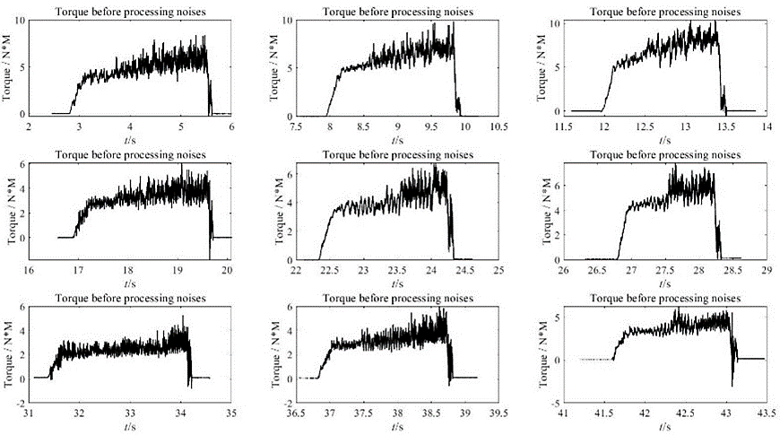
Figure 12. 9 sets of torque data before processing noises.

The data in this section was sliced and enlarged in order for not only the thrust and torque changes to be more clearly viewed, but also the distribution of noise and the actual measured values to be intuitively understood in this section.

There are further advantages to slicing data. For example, the stability of test results, the distribution of observation data, and soon. In this experiment, the data was split in order to study the borehole's features independently of one another.

The same may be said about changes and relationships between distinct sets of data, which can be detected via the use of different data images. As a result, the effect of high speed and high feed output on thrust has been confirmed once again. The data collected in our experiment was not steady and there was a lot of noise, as described above in the description of data slices. This information was useful in our next step, which was to analyse the data.

4.3. Thrust and torque after processing noises

According to the section diagram Fig 10, we may conclude that the measured data comprises a variety of noises, which may be from the power supply, the machine itself, or the lines that link the data acquisition equipment to the data collection device. Referring to the noise removal method in the experimental method, MATLAB will fit a curve through the data and plot a line, this term will process as much data as possible to achieve better approximation, especially when there are lots of noisy samples, this means will give a better approximation. The following thrust diagram after noise removal is obtained:

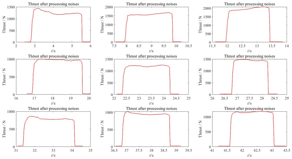
Figure 13. 9 sets of thrust data after processing noise.

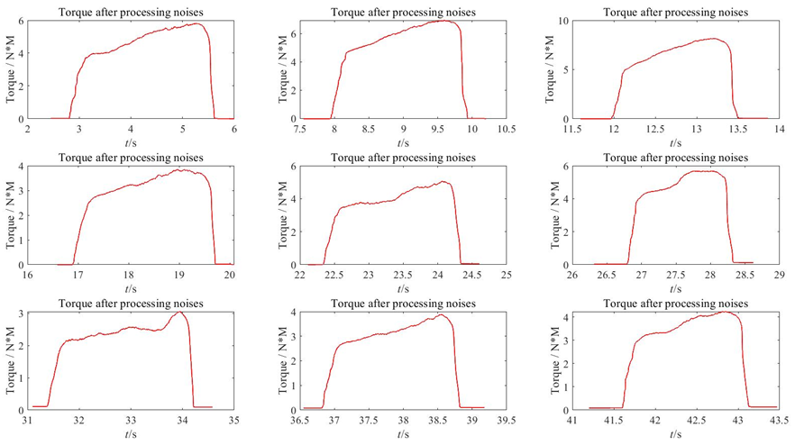
Figure 14. 9 sets of torque data after processing noises.

At the very beginning of this experiment, we want to measure the red line in figure 13 and 14, which represents the stable and real signal, but what we actually measure and get is the black line in figure 10 which mainly because of noises. The greater the number of samples we gather and include in our average, the closer and better our estimate of the genuine value becomes. To achieve a smooth line like this, we must analyse a large number of additional samples; thus, having a pot like this will indicate if it is worthwhile to continue collecting data, because more data means more time and money.

For noise removal, we first think of the three-point mean method, which is the following formula:

\( y(n)=\frac{y(n-1)+y(n)+y(n+1)}{3} \)

However, this method cannot eliminate the noise fundamentally, and will only mix the noise with the experimental value, so the effect is not obvious. Secondly, the three- point averaging method is generally only applicable to the single-frequency noise system, which is contrary to the experiment. So that was ruled out.

The essence of noise removal is to retain the DC voltage, remove the AC voltage. According to the procedure of the experiment, finally we remove the noise and get closer to the actual measurement.

4.4. Generate thrust frequency spectrum

The result of this experiment is the single-sided power spectrum processed by FFT. The following figure shows the distribution of thrust and torque power at each frequency point, reflecting the change of power with frequency.

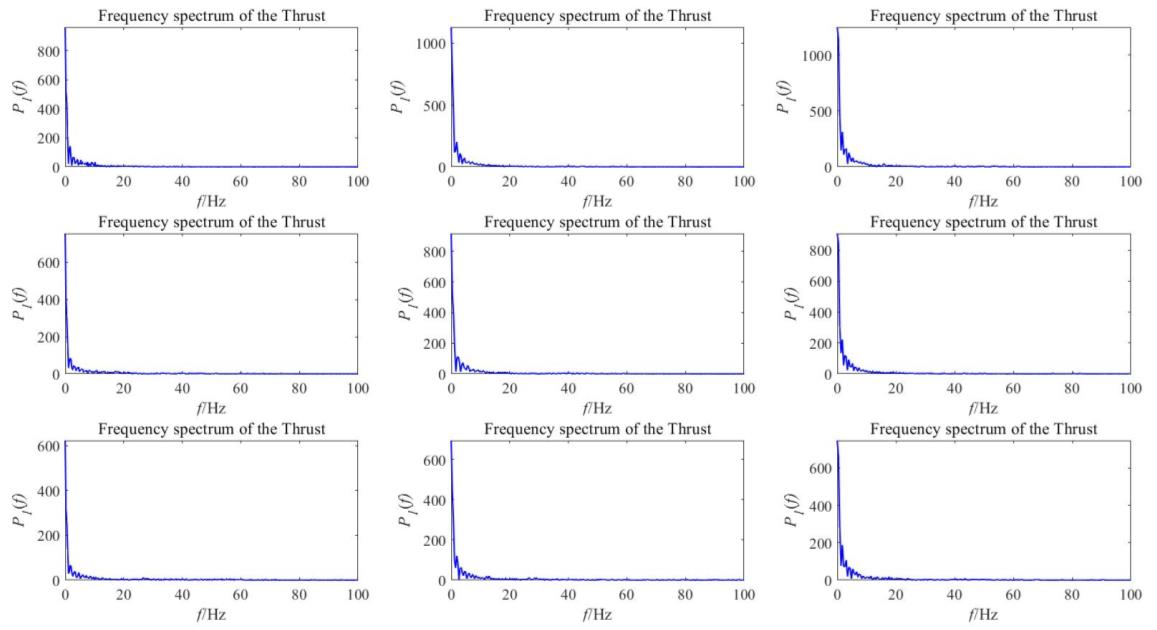
Figure 15. Thrust frequency spectrum.

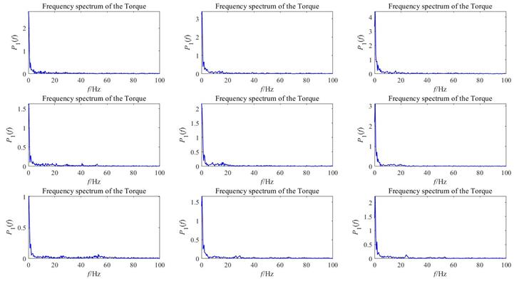
Figure 16. Torque frequency spectrum.

From the power spectrum results, it is found that the peak appears at the first 0 Hz, and then rapidly decreases and stabilizes. Since the power has no negative value, the power spectrum curve is only close to zero in the end. Thearea of the power spectrum can represent the total power of the signal. It is obvious that the total power of the thrust signal is much greater than that of the torque.

4.5. Mean value and standard deviation of thrust

Sample standard deviation, also known as experimental standard deviation: For sampling from a population, using a sample to calculate the population deviation. After calculating the mean value, the standard deviation equation can be established, as shown below:

\( {S_{X}}={[\frac{1}{N-1}\sum _{i=1}^{N}{({X_{i}}-X)^{2}}]^{2}} \)

The following table of standard deviation and mean can be obtained from the above formula:

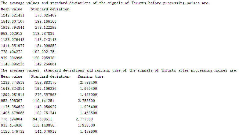
Figure 17. Mean value and standard deviation of thrust.

By comparing the standard deviation table before and after noise elimination, we can clearly see that the table after noise elimination has a higher degree of convergence. The error is almost negligible, within 5%. This further validates the accuracy of our noise removal, and also shows that the value after noise removal is closer to the actual value.

4.6. Curve fit

According to the average value of thrust, we constructed linear regression equations of thrust and speed, thrust and feed through MATLAB. The results are as follows:

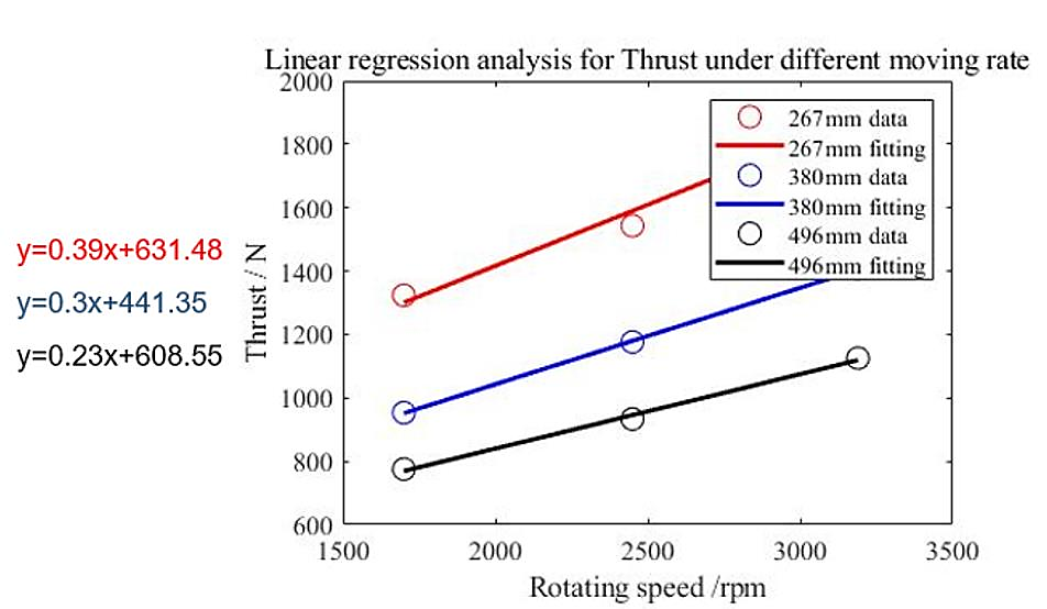
Figure 18. Thrust and moving rate.

It is observed that, on the whole, as the rotational speed increases, the thrust also increases. At the same speed, the greater the feed, the smaller the thrust.

The following is a linear regression diagram of feed and thrust:

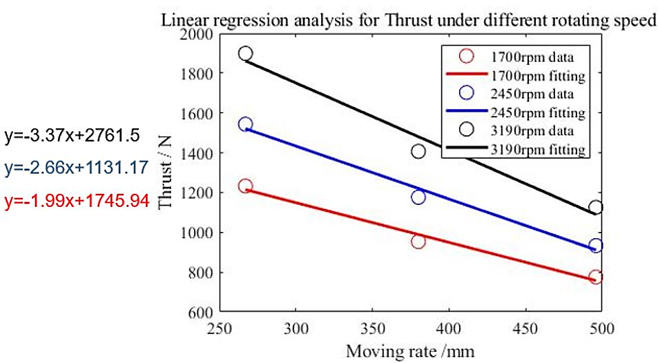
Figure 19. Thrust and rotating speed

According to the linear regression diagram of thrust and feed, it can be seen that the collected thrust decreases with the increase of feed.

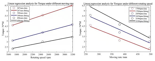
Figure 20. Linear regression analysis for Torque under different moving rate and rotating speed.

Figure 20 shows under different moving rate and rotating speed , the linear regression analysis for torque. Torque increases with the increase of rotating speed, which shows a positive proportional linear correlation. On the right-hand side, torque decreases with the increase of moving rate, which means they have a negative proportional linear correlation.

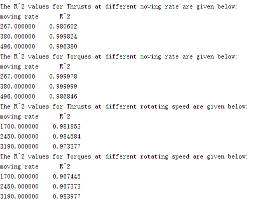
Figure 21. r2 for thrusts and toques.

r2 represents how good the curve fitting, the closer it is to 1, the better, in this case , it is really good.

4.7. Compare and evaluate movmean and movmedian

Knowing how to communicate, what methods to utilize, and what to do with the data once we collect it is one of the most important subjects and major reasons for carrying out this project.

To compare and evaluate movmean and movmedian, change command from movdedian to movmean for thrust and torque.

F_sub2=smoothdata(F_sub, 'movmean'); %smoothing andNoise reduction

Figure 22. Movmean command for thrust.

Figure 23. Movmean command for torque.

In figure 16, the first graph on the left-hand side is the graph of thrust we got using movmean, right hand side is graph of thrust using movdedian.

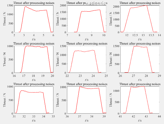
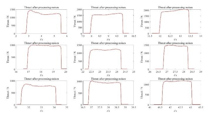
Figure 24. 1 Movmedian and movmean comparisan of thrust.

Correspondingly, in figure 24, the first graph is the graph of torque using movmean, and second is graph of thrust using movdedian.

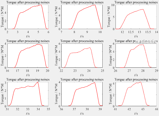
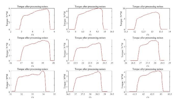
Figure 25. Movmedian and movmean comparisan of torque.

In comparisan, movdedian is a better data process approach. The slope of the curve at the beginning and ending are greater. In real and ideal situation, the data should change abruptly when the drill starts working and contact begins, graphs should go up and down vertically, so movmedian approach is closer which means better for processing this data.

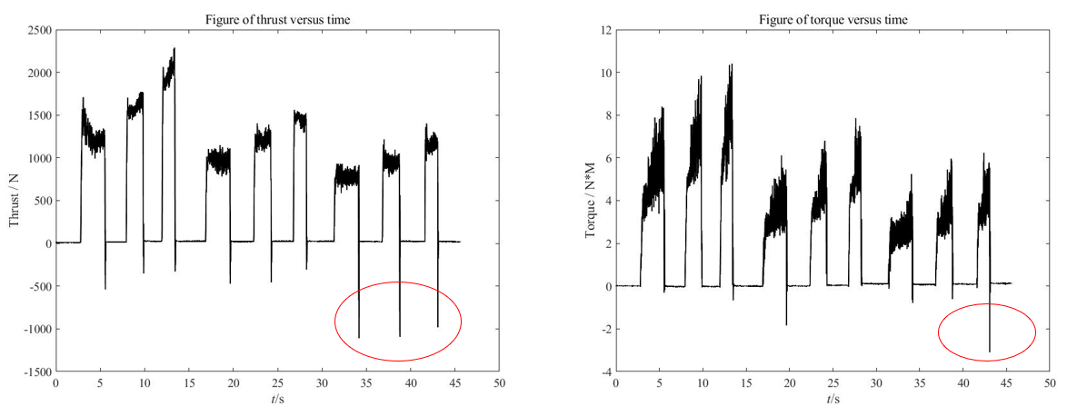
Figure 26. Thrust and Torque verses time.

The average included and processed all of the noise data, as a result, it is farther away from the real value. In skewed distributions, the median is a highly frequent and valuable statistic that may be used to compensate for the shortcomings of the mean statistic. In the case of the mean, we know that a change in any of the values in the sample will have an impact on the final computation, and that in the case of a large outlier change in one of the values(noises), the mean may fail. In figure above, noise data is marked and that is obviously irrelevant. The median method is more accurate because it eliminates the effect of those extreme values. Graphs using movdedian approach processed data are quite smooth.

4.8. Data mutation area and manufacturing process

Figure 27(a) is a typical fluctuation in the original thrust data. It can be clearly found that a large fluctuation occurs when the turning tool starts to process a hole, and the back force has a slight decrease trend. However, after the tool is retracted, a larger reverse thrust is measured.

Cheng.H.D studied this phenomenon and proved that the thrust of the hole is related to the diameter of the hole. Figure 27(b) shows that the thrust will gradually decrease when the hole diameter increases, and this trend is similar to they=-ln(x) curve. When the drill bit just touches the workpiece, the hole diameter will change from 0 to the machining diameter. Therefore, a larger thrust can be generated, similar to the phenomenon of stress concentration. When the drill is retracted, the drill will move vertically and reversely. Due to the influence of chips and processing dimensions, the workpiece will also have a tendency to follow the movement of the turning tool. Therefore, the sensor can measure a reverse thrust.

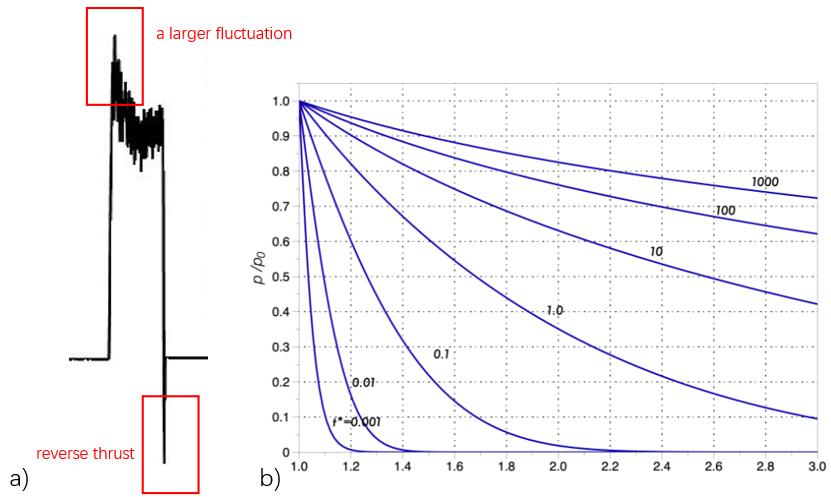
Figure 27. Raw data of a thrust (a), Cheng.H.D's numerical results (b).

In addition, these mechanical behaviours should not exist under ideal conditions. The thrust map after noise removal also shows a shape similar to a square wave. These mechanical changes are removed, especially the reverse thrust, and the square wave is actually an ideal thrust image.

Compared with thrust, the torque fluctuation in the original data is simpler. As the drilling depth increases, the torque gradually increases. Zhongliang studied the impact of drilling depth and feed rate on the torque of the drill bit[2]. When the drilling depth increases, the increase in friction caused by the residual cutting accumulation will cause the torque to increase. This is also one of the main reasons for the fracture of the turning tool. Therefore, it is necessary to consider the change of the drilling depth in the processing and manufacturing, and the tool can be retracted during the drilling and the chips can be cleaned to continue processing.

5. Future recommendations

In the LabVIEW program part, the FPGA is used to record data at a high frequency and uses TDMS format to accurately record data. In terms of recording data, it is expected that the signal and time from the CNC machine will be recorded in one TDMS file at the same time. However, due to the problem of the data format, the recording time is too long, and the time recorded in the file exceeds the upper limit of storage and abnormal numbers (negative numbers, etc.) appear. This may be improved by changing the data format and optimizing the structure of the program. In MATLAB section, the code can be optimized by further studying.

In addition, since the value of force recorded by the MyRio device is not a direct force value, some mathematical transformation is needed to convert the data into the required force. In this project, MATLAB was used to complete this work. Consider completing part of the primary transformation in LabVIEW. This may be accomplished by adding a series of operations to the host program.

6. Conclusion

This report presents and discusses the process, methodology and results of the project in five parts. The first section provided the research background of the project and sets the objectives. In the second section, the methods used in the experimental, LabVIEW and MATLAB sections are described in detail. The third section showed and discussed the results after processing. The

fourth section offered suggestions for the next steps in future work. The final section summarized the contents of the report.

References

[1]. An, S., He, Y., Qian, R. and Liu, X., 2011. Study for Vibration Measurement and Failure Diagnostics System for CNC Milling Machines Based on LabVIEW. Advanced Materials Research, 189-193, pp.1180-1183.
[2]. Detournay E, Cheng AHD. Poroelastic response of a borehole in anon-hydrostatic stress field. International Journal of Rock Mechanics and Mining Sciences & Geomechanics Abstracts. 1988;25:171-82.
[3]. MathWorks, 2021. Moving median - MATLAB movmedian- MathWorks China. [online] Ww2.mathworks.cn. Available at: <https://ww2.mathworks.cn/help/matlab/ref/movmedian.html?lang=en> [Accessed 16 December 2021].
[4]. Milfelner, M., Cus, F. and Balic, J., 2005. An overview of data acquisition system for cutting force measuring and optimization in milling. Journal of Materials Processing Technology, 164-165, pp.1281-1288.
[5]. Kalpakjian, S. and Schmid, S., 2017. manufacturing process for engineering materials. 6th ed.
[6]. Stavropoulos, P., Chantzis, D., Doukas, C., Papacharalampopoulos, A. and Chryssolouris, G., 2013. Monitoring and Control of Manufacturing Processes: A Review. Procedia CIRP, 8, pp.421-425.
[7]. Sun, I. and Chen, K., 2017. Development of signal transmission and reduction modules for status monitoring and prediction of machine tools. 2017 56th Annual Conference of the Society of Instrument and Control Engineers of Japan (SICE) ,.
[8]. Yeh, S. and Chen, C., 2021. Integrated Design of Spindle Speed Modulation and Cutting Vibration Suppression Controls Using Disturbance Observer for Thread Milling. Materials, 14(21), p.6656.
[9]. Wei Zhongliang CT. Research on Factors Affecting Torque During PDC Bit Drilling. Oil drilling technology. 1995;1.
[10]. Ww2.mathworks.cn. 2021. Fast Fourier Transform - MATLAB fft- MathWorks China. [online] Available at: <https://ww2.mathworks.cn/help/matlab/ref/fft.html> [Accessed 17 December 2021].
Cite this article
Xu,Y. (2024). Virtual instrumentation-based data collection and analysis for CNC machining process. Applied and Computational Engineering,62,15-32.
Data availability
The datasets used and/or analyzed during the current study will be available from the authors upon reasonable request.
Disclaimer/Publisher's Note
The statements, opinions and data contained in all publications are solely those of the individual author(s) and contributor(s) and not of EWA Publishing and/or the editor(s). EWA Publishing and/or the editor(s) disclaim responsibility for any injury to people or property resulting from any ideas, methods, instructions or products referred to in the content.
About volume
Volume title: Proceedings of the 2nd International Conference on Mechatronics and Smart Systems
© 2024 by the author(s). Licensee EWA Publishing, Oxford, UK. This article is an open access article distributed under the terms and
conditions of the Creative Commons Attribution (CC BY) license. Authors who
publish this series agree to the following terms:
1. Authors retain copyright and grant the series right of first publication with the work simultaneously licensed under a Creative Commons
Attribution License that allows others to share the work with an acknowledgment of the work's authorship and initial publication in this
series.
2. Authors are able to enter into separate, additional contractual arrangements for the non-exclusive distribution of the series's published
version of the work (e.g., post it to an institutional repository or publish it in a book), with an acknowledgment of its initial
publication in this series.
3. Authors are permitted and encouraged to post their work online (e.g., in institutional repositories or on their website) prior to and
during the submission process, as it can lead to productive exchanges, as well as earlier and greater citation of published work (See
Open access policy for details).