1 Introduction

In contemporary computing architectures, Reinforcement Learning (RL) is recognized as a critical subfield of machine learning [1]. Distinct from traditional supervised and unsupervised learning approaches, which aim to uncover latent data structures or predict outcomes for new data, RL does not seek a singular "correct" answer. Instead, its goal is to optimize outcomes through trial and error, striving to secure the best possible rewards or strategies. This branch of machine learning holds significant potential and has seen diverse applications. For instance, in the realm of gaming, RL influences everything from traditional board game strategies, such as chess, to the development of modern video games. In robotics, it accelerates iteration and updates, enabling robots to adapt more effectively to their environments. RL also plays a role in enhancing recommendation systems and the functionality of conversational AI [2].

The fundamental elements of reinforcement learning include agents, environments, actions, and rewards. The primary objective is to assist agents in discovering the most effective strategy to maximize cumulative rewards.

The basic model of Reinforcement Learning (RL) can usually be described by a Markov Decision Process (MDP). Reinforcement learning problems can generally be represented by four-tuple . S represents the set of all states s. A represents the set of all actions for every s in S. P represents the set of transition probability, which means that the probability of an agent transitioning from s to s' via action a, and its main expression is P (s, a, s') or P (s'| s, a). R represents the set of immediate reward, which means the immediate reward obtained by the agent in s is to move to s through action a, and its expression is R (s, a, s'). If we want to briefly represent this tuple, this can be simplified to . T (s, a, s') represents the transition function which combines the transition probability and the immediate reward, and contains the probability and reward of s transferring to s’ through action a. Generally, reinforcement learning methods are mainly divided into two categories: Model-based Learning and Model-free Learning. Model-Based reinforcement learning methods involve building a model of an environment, trying to understand the transfer equation T of the environment. This model \( \hat{T} \) can be given in advance or learned through interaction with the environment. Using this model, agent can predict the consequences of their actions, plan and make decisions. Model-Free reinforcement learning methods do not directly build a model of the environment. Instead, they learn how to achieve their goals by interacting directly with their environment. Model-Free methods focus on learning a policy \( π \) (s, a) or value function V (s) or Q (s, a). As shown in Figure 1.

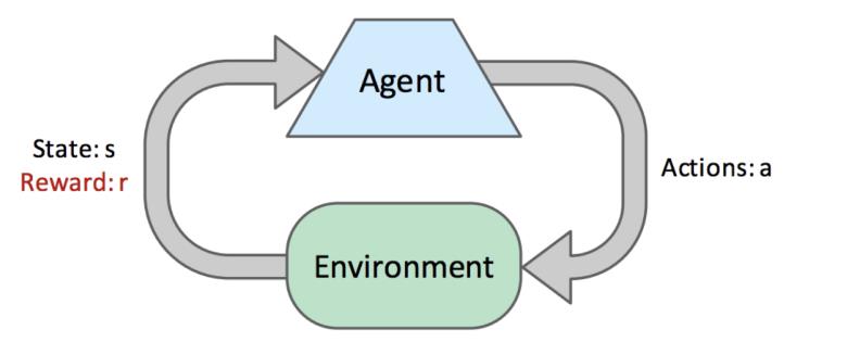Figure 1. Reinforcement Learning process (Photo/Picture credit: Original).

Multi-armed Bandit problem is a type of reinforcement learning, but it is not a typical reinforcement learning problem because the agent and the environment do not interact [3]. It is a sequential learning process like reinforcement learning, but it is not Cannot change the distribution of rewards or the content of the environment. Its purpose is also very similar to RL, which is to maximize the cumulative reward, but in experiments this is more transformed into minimizing the cumulative regret. Compared with traditional reinforcement learning problems, its application is more subdivided and focused more on Various recommendation systems, such as movies, books, etc., have a certain impact on financial investment, agriculture, and clinical medical experiments.

The main purpose of the MAB algorithm is to minimize the cumulative regret in the process by balancing the exploration and exploitation dilemma in long-term consequences. Nowadays, the MAB algorithm has made rapid progress, and they have different parameters. That is, the number of arms, the number of rounds, or the reward distribution have different performances. There are many types of MAB problems, the most basic of which is the stochastic stationary bandit problem. This article hopes to simulate the process of these algorithms in the stochastic stationary multi-armed bandit problem as much as possible by changing different data sets to complete comparative analysis. For algorithms with deterministic parameters, optimize their performance by adjusting and optimizing the parameters. This may help to find suitable MAB algorithms more quickly in future research in different directions, in order to provide certain reference in different fields.

2 Relevant Theories

2.1 Definition and Development of Multi-armed Bandits

2.1.1 Conceptual Framework. The model of Multi-armed Bandits could be represented by 3-tuple . Since the multi-armed bandit problem does not interact with the environment, compared to the reinforcement learning problem, there is no need to record the environmental state S. |A| = k and A = { \( a_{1},…, a_{k} \) }, which represents the set of all actions. Because actions cannot have an impact on the environment, there is no need to define actions for each state, but it is necessary to focus on defining the round t. t \( ∈ \) N, N here represents horizon, a value that we can define before the experiment starts. Usually, this is the total number of actions the agent takes. Every time the agent takes an action, the value of t will be increased by 1. When t reaches N, the experiment stops. \( r_{a, t} \) \( ∈ \) R, which represents the actual reward obtained by acting a in round t. However, in general, for an action, that is, an arm, a deterministic reward is usually not obtained. This is usually based on to determine the distribution of rewards. For example, for clicks on advertising, in actual situations, the agent will collect two reward values ​​0 or 1 from the action \( a_{i} \) . \( p_{i} \) represents the probability of reward 1 and 1 - \( p_{i} \) represents the probability of reward 0. Hence, E [ \( r_{i} \) ] = \( p_{i} \) , E [ \( r_{i} \) ] represents expected value of the reward from action. In literature, to explore the MAB problem, it is usually not measured directly by the actual rewards obtained, but by average expectations. Q is the set of average expectations of rewards in rounds t. Hence, \( Q_{t}(a)=E[r_{t}a] \) . The existence of Q helps the design of the algorithm, because it can record the rewards we obtained for each arm before round t+1 to provide support for the decision-making at t+1. For the learner itself, the purpose is Maximize the total value of reward in N rounds.

\( S_{n}= \sum_{t=1}^{n} r_{t } \) (1)

In other words, for the MAB problem, the learner's goal can be transformed into minimizing cumulative regret R. Because the MAB problem does not interact with the environment, it can be used as the learner's goal in a more convenient way to analyze. Such a formula can make it easier to see the gap between the experimental process and the optimal situation, which facilitates subsequent research in order to put it into real application scenarios.

\( R =\sum_{t=1}^{n} r_{t}^{*}-\sum_{t=1}^{n} r_{t} \) (2)

Here, \( r_{t}^{*} \) represents the actual reward of the largest possible arm in each round. In actual situations, the value of r is determined based on the distribution. In experiments, the situation will be more focused on the use of average expectations, which can provide overall support for the experimental results. Here, u* represents the average expectation of the best arm if we know. \( π \) presents the policy. \( E[\sum_{t=1}^{n} r_{t}] \) represents the expected cumulative reward of our policy.

\( R(π) =n * u^{*}-E[\sum_{t=1}^{n} r_{t}] \) (3)

The most classic and direct case of the Multi-armed Bandit problem is the selection of slot machines in casinos. If a person has a capital F and the cost per use of each slot machine is c, then N in the MAB problem is \( F/c \) , and he wants to maximize his net income from the casino. In the traditional A/B testing method, people test all slot machines that can be invested in set rounds. If the test phase is longer, it will indeed have higher confidence for the winner, but it will also cost more money. That is, resources are wasted exploring unimportant options. After the exploration phase is over, the experiment will suddenly drop into the utilization phase. However, in more MAB algorithms, people have found more ways to balance the dilemma of exploration and utilization, which also promotes the development of MAB algorithms.

2.1.2 Evolution and Types of Multi-Armed Bandits. Due to the application of MAB in various modern directions, its iterations have gradually come into people's vision. To be more relevant from the perspective of practical application, people have also subdivided it into several important categories and gradually divided it into these several directions for research. Accordingly, the MAB algorithm in the traditional sense has also adopted certain adjustments and changes on these issues. According to different natures, researchers divide conceptual MAB problems into the following types of problems, which add more restrictions or conditions than the content of the actual problems.

The first is stochastic stationary Bandits, which is also the main content discussed in this article. Similarly, it is also the core content of the MAB problem. Basically, all algorithms are born based on this problem, and then under the conditions of other types of MAB to adjust and analyze. Its core is that the reward of each arm of r comes from their fixed reward distribution, which is linked to their actions, and will not change according to the increase of rounds, that is, the change of time, which represents the characteristics of stationary, and the reward obtained by each action is randomly obtained according to the distribution. According to this characteristic, the researcher can simplify the process of extracting the arm's reward. It no longer directly extracts the reward from the data set based on the arm's serial number but use storage distribution to simplify the reward acquisition process.

The second category is Non-Stationary (Restless) Bandits, whose characteristics correspond to Stochastic Stationary Bandits. Similarly, the agent cannot affect the environment through actions, but the environment will gradually change as t increases, which is reflected in the randomness of the reward distribution. With the change of time, this requires the traditional stochastic stationary algorithm to introduce more considerations about the time round t.

Next is Structured Bandits. The main feature of this type of problem is that it assumes that there is a clear structure existing in the reward distribution, which affects the entire problem process. Such an assumption can make the execution process of the algorithm have more suitable parameters, help the algorithm better predict the distribution of the entire reward, and optimize the purpose of the experiment, which is to minimize cumulative regret. Expressing it as a formula, there are two types of expressions: Linear Bandits and Global Structured Bandits.

\( r_{t} =a * θ + η_{t} \) (4)

\( r_{t} \) is a linear function here with respect to \( θ \) . This is also the main definition of Linear structured Bandits. \( θ \) is the core of the problem of structured bandits. It is an unknown universal parameter that has an impact on all arms. a is a known parameter for all actions. It is similar to the weight of approximate Q learning and reflects the difference between different actions. \( η_{t} \) is a noise variable, which has a known distribution and is used to reflect the uncertainty of the action. Another way to define it is Global Structured Bandits, or it is an expansion of Linear Bandits. The reward received by an action is not defined by a simple linear expression. Instead, use arbitrary function to represent.

\( r_{t}=f(θ;a) \) (5)

Another type of MAB is Correlated Bandits, which assumes that the rewards of different arms are related to each other. This connection requires us to have more prior knowledge. At the same time, this assumption also allows researchers to better improve the algorithm performance. For example, in a recommendation system, when advertisements are placed, the target group is mostly book lovers, so the reward distribution between several advertisements about reading content may have a great correlation, for example, their average click-through rates will all be the same. is very high, or if the two advertisements are very close to each other when choosing where to place the ads, then their reward distributions may also be relatively similar.

Regarding the expansion of MAB, another very popular and important category is Contextual Bandits. The difference in its definition is that before taking an action at each round, learner receive a “side information” or “context” about the current state of the environment. Under this circumstance, overtime, the goal is to learn the best action for each context. This allows the learner to obtain more information to improve his performance. Under this assumption, it will have better results for the performance of the experimental target. For example, in the recommendation system, it can make use of the user's age, hobbies and other characteristics. This is very similar to the characteristics of machine learning, but it is not to make predictions, but to make better strategies.

2.2 Fundamental Concepts of Stochastic Stationary Bandits Problems

2.2.1 Cumulative Regrets and Its implications. Under the above concept, researchers need to clarify the definition of stochastic stationary bandits. Stochastic Stationary Bandits Problems have a set of available actions or arms A, and each action a \( ∈A \) is associated with a reward distribution \( P_{a} \) . In each round t = 1, 2, …, n, the learner chooses an action \( a_{t}∈A \) and receives a reward \( r_{t} \) that is sample from \( P_{A_{t}} \) . Then, typically, there are some knowledge on the distributions ( \( P_{a}: \) a \( ∈A) \) which is called the environment class.

Since in the literature, researchers pay more attention to the average reward because it contains more information, the average reward for each arm should be defined like this.

\( u_{a}= \int_{- ∞}^{∞} x*dP_{a}(x) \) (6)

\( u_{a}=E[X_{t}A_{t}=a] \) (7)

(6) is the mean value of a continuous mean reward whose distribution is \( P_{a}. \) (7) is the conditional mean of reward learner receive in round t give that learner choose arm a in round t.

(7) could be rewritten like this.

\( u_{a}= \sum_{x}^{} P(r_{a}=x)*x \) (8)

To correctly define the cumulative regret of stochastic stationary bandits, best arm, that is the arm with the largest mean reward.

\( a^{*}= arg \max{a ∈ A}{u_{a}} \) (9)

Here, \( a^{*} \) sometimes is denote by \( k^{*} \) . It’s the index of the best arm. For example, it’s the advertisement version with the highest click-rate in advertising recommendation system.

\( u^{*}= \max{a ∈ A}{u_{a}} \) (10)

\( u^{*} \) is the largest mean reward of all arms. In the above example. It’s the largest click rate of all advertisement versions. In this way, the cumulative regret of stochastic stationary bandits can be defined as follows.

\( R_{n}(π) =n * u^{*}-E[\sum_{t=1}^{n} r_{t}]R_{n}(π) \) is the expected regret of policy \( π \) accumulated in n rounds. \( n * u^{*} \) is the expected cumulative reward researchers would have gotten if they knew which arm was the best. Then, the learner’s goal is to minimize \( R_{n}(π) \) .

2.2.2 The Concept of Logarithm Regret. In this case, how to measure what a good algorithm is to first define the logarithm regret. Before defining the logarithm regret, sub-linear regret should be defined clearly.

\( \lim{n→∞}{\frac{R_{n}}{n}} \) = 0 (11)

\( R_{n}=o(n) \) (12)

This means that the algorithm chooses the best action almost all the time in the limit of horizon n going to infinity. The learner can usually do better than regret being just sub-linear under the algorithm.

\( R_{n}≤C*log{n} \) (13)

\( R_{n}=O(log{n}) \) (14)

For better understanding of logarithmic regret of Stochastic Stationary Bandits Problems, the significance of regret as a logarithm to the number or frequency of suboptimal decisions plays a decisive role. To figure out this, regret decomposition should be defined. First, express the regret term in (11) in terms of the number of sub-optimal choices.

\( T_{a} (t)= \sum_{i=1}^{t} I [a_{i}=a] \) (15)

For any a \( ∈A \) , let \( ∆_{a}= u^{*}- u_{a} \) define the sub-optimality gap of action a. It’s the difference between the mean reward of the best action and the mean of action a. For the best arm \( a^{*} \) , the sub-optimality gap is 0, that is, \( ∆_{a^{*}} \) = 0. Then, regret can be rewritten as below.

\( R_{n}= \sum_{a ϵ A}^{} ∆_{a}*E[T_{a} ( n )] \) (16)

\( ∆_{a} \) is the regret incurred each time action a is taken. \( E[T_{a} ( n )] \) is the mean number of times action a is taken in n rounds. Then, the goal of the learner is to minimize the weighted sum of expected action counts, where the weights are equal to the sub-optimality gaps. The learner should try to choose an arm with a larger \( ∆ \) proportionally fewer times. \( R_{n} \) is logarithmic, that is \( R_{n} \) = O (log n), if and only if \( E[T_{a} ( n ) \) ] = O (log n) for all sub-optimal arms a = \( a^{*} \) .

\( E[T_{a} ( n )]= \sum_{t=1}^{n} P (a_{t}=a) \) (17)

If \( \sum_{t=1}^{n} P (a_{t}=a) \) = O (log n), there should be (17)

\( P( a_{t}=a )≅ \frac{1}{t} \) (18)

\( \frac{1}{t} \) follows intuitively from \( \int_{}^{} \frac{1}{x}dx=log⁡(x) \) . Logarithmic regret is achieved if the probability that the algorithm makes a sub-optimal decision in round t decays as \( \frac{1}{t} \) .

2.2.3 Exploration-Exploitation Trade-off. According to the characteristics of MAB, the environment does not reveal the reward of the actions not selected by the learner, that is, the learner should gain information by repeatedly selecting all actions to exploit. When the learner selects a sub-optimal action, it loses from the cumulative reward. The learner should try to exploit the action that returned the largest reward so far. The important part of the MAB algorithm is the balance of these two parts, which is also an important feature that distinguishes them from the A/B testing method. How to accurately understand these two parts and reasonably optimize the structure and function of these two parts can achieve the goal of the learner.

2.3 Implementation of Different Algorithms

2.3.1 Explore-Then-Commit (ETC). The core of this algorithm is like A | B testing method. ETC algorithm is to explore by playing each arm a fixed number of times and then exploits by committing to the arm that appeared the best during exploration. And it could be assumed that the reward distribution for all arms is 1-subGaussian ( \( τ \) – sub-Gaussian with \( τ \) = 1). That is, for any \( τ \) \( ≥ \) 0, a random variable X being 1-subGaussian means that

\( P(X≥ τ) ≤ e^{-\frac{τ^{2}}{2}} \) (19)

Here, \( P(X≥ τ) \) is the tail probability of X. \( e^{-\frac{τ^{2}}{2}} \) is the tail probability of a Gaussian random variable with mean = 0 and variance = \( τ^{2} \) = 1 (Normal Distribution). As shown in Figure 2.

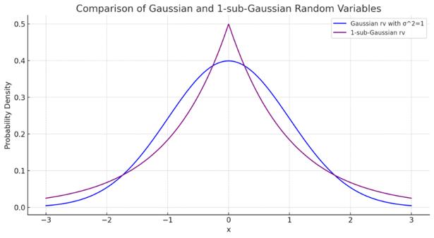Figure 2. Comparison of Gaussian and 1-subGaussian (Photo/Picture credit: Original).

If x is bounded in the interval [a, b], then x is \( τ \) – subGaussian with \( τ \) = \( \frac{b - a}{2} \) .

The ETC algorithm assume there are k arms. Let me: number of times each arm will be explored.

Algorithm 1 ETC

procedure ETC (N, m, k)

Input m

For each t = 1, 2, … choose action

\( A_{t} \) = \( \begin{cases}(t mod k)+1, if t ≤m*k arg{\max{i}{\hat{u}_{i}(m*k), if t ≥}} m*k\end{cases} \) (20)

(Where \( \hat{u}_{i} \) (t) = \( \frac{\sum_{s=i}^{t} 1[A_{s} = i] X_{s}}{\sum_{s=i}^{t} 1[A_{s} = i] } \) ).

Store \( R_{n} \) .

Continue.

Return cumulative regret.

Here \( \sum_{s=i}^{t} 1[A_{s}=i]X_{s} \) represents total reward from i until round t. \( \sum_{s=i}^{t} 1[A_{s}=i] \) represents the number of times arm i is selected until round t, which equals to \( T_{i} \) (t)

The exploration phase of ETC phase is choosing each arm in a round-robin fashion until all k arms are selected m times each. And the exploitation or commit phase is starting with round t = m * k + 1, the algorithm selects the arm with the largest average reward in the exploration phase for all future rounds.

The regret in exploration phase is the formula below.

\( R_{(exploration)} = \sum_{i = 1}^{k} ∆_{i} * m \) (21)

In the commit phase,

\( R_{(exploitation)} = (n-m * k) * \sum_{i = 1}^{k} ∆_{i} * P (\hat{u}_{i}(m * k) ≥ \max{j ≠ i}{\hat{u}_{j}(m * k)}) \) (22)

\( P (\hat{u}_{i}(m * k) ≥ \max{j ≠ i}{\hat{u}_{j}(m * k)} \) is the probability of committing to arm i in all these n – m * k rounds. Let \( ∆_{1} \) = 0 (let arm 1to be the optimal arm) without loss of geniality.

\( R_{(exploitation)} = (n-m * k) * \sum_{i = 2}^{k} ∆_{i} * P (\hat{u}_{i}(m * k) ≥ \max{j ≠ i}{\hat{u}_{j}(m * k)}) \) (23)

Next, this could simply lead to the below formulation.

\( R_{n}≤ m * \sum_{i = 1}^{k} ∆_{i}+ (n-m * k) * \sum_{i = 2}^{k} ∆_{i} * P (\hat{u}_{i}(m * k) ≥ \hat{u}_{1}(m * k)) \) (24)

When the reward distributions are 1-subGaussian, there is.

\( P(\hat{u}_{i}(m * k) ≥ \hat{u}_{1}(m * k)) ≤ e^{-\frac{m * ∆_{i}^{2}}{4}} \) (25)

So, this lead to (23).

\( R_{n} ≤ m * \sum_{i = 2}^{k} ∆_{i}+ (n-m * k) * \sum_{i = 2}^{k} ∆_{i} * e^{-\frac{m * ∆_{i}^{2}}{4}} \) (26)

(23) illustrates the trade-off between exploration and exploitation.

If the researcher chooses the large m. The second term \( (n-m * k) * \sum_{i = 2}^{k} ∆_{i} * e^{-\frac{m * ∆_{i}^{2}}{4}} \) is going to be very small. But the first term \( m * \sum_{i = 1}^{k} ∆_{i} \) will be large. Hence, how to choose m decides regret. First, assume that k = 2, then \( ∆_{1} \) = 0, \( ∆_{2} \) = \( ∆ \) . With this simplification, (23) becomes the formulation below since n – m * k \( < \) .n.

\( R_{n} ≤ m * ∆ + ∆ * e^{log (- \frac{m * ∆^{2}}{4})} \) (27)

\( e^{log (- \frac{m * ∆^{2}}{4})} \) \( ≤ \) 1 if \( \frac{m * ∆^{2}}{4} \) \( ≥ \) log n, which means that researcher can make second term less than \( ∆ \) which is the regret incurred by each sub-optimal choice.

\( m = ⌈\frac{4 * log n}{∆^{2}}⌉ \) (28)

With this choice, it could lead to (26)

\( R_{n} ≤ \frac{4 * log n}{∆} + 2 * ∆ \) (29)

With \( ∆ \) > 0, \( R_{n} \) = O (log n).

While the researcher use more than 2 arms (k is arbitrary), m need to change its expression. This need to have (27).

\( m = ⌈\frac{4 * log n}{\min{i ≠ 1}{∆_{i}^{2}}}⌉ \) (30)

Which gives a regret of (28).

\( R_{n} \widetilde{≤} ⌈\frac{4 * log n}{\min{j ≠ 1}{∆_{j}^{2}}}⌉ * \sum_{i = 2}^{k} ∆_{i} + η \) (31)

\( η \) is small terms that do not depend on n. (25) requires knowledge of \( ∆ \) and n. To make m data independent, that is, algorithm keeps exploring until the observed data meets certain conditions.

\( |\hat{u_{1}}(2*m)-\hat{u_{2}}(2*m)|≥threshold(canbeafunctionofm) \) (32)

With this approach, it was shown that it is possible to achieve \( R_{n} ≅ \frac{4 * log n}{∆} \) .

2.3.2 Upper-Confidence-Bound (UCB). The point where the ETC algorithm can be improved is that researchers need the advance knowledge of the sub-optimality gaps and there is an abrupt transition from exploration phase to exploitation phase.

The main idea of the UCB algorithm is based on the principle of optimism under uncertainty. It is, in each round, assign a value to each arm (called the UCB index of that arm) based on the data observed so far that is an overestimate of its mean reward (with high probability), and then choose the arm with largest value 1 index.

\( UCB_{i} ( t-1 )= \hat{u}_{i}( i-1 )+Exploration bonus \) (33)

\( UCB_{i} ( t-1 ) \) is the UCB index of arm I in round i – 1, and \( \hat{u}_{i}( i-1 ) \) is the average reward from arm I till round t – 1. \( Exploration bonus \) is a decreasing function of \( T_{i} ( t-1 ). \) \( T_{i} ( t-1 ) \) is the number of samples obtained from arm I so far. So, the fewer samples we have for an arm, the larger will be its exploration bonus. Being optimistic about the unknown support exploration of different choices, particularly those that have not been selected many times. The exploration bonus should be large enough to ensure exploration but not so large that sub-optimal arms are explored unnecessarily.

\( \hat{u}= \frac{\sum_{t=1}^{n} X_{t}}{n} \) (34)

\( P(\hat{u}+ \sqrt[]{\frac{2log{(\frac{1}{δ})}}{n}}>u)≥1- δ for all δ ∈(0,1) \) (35)

\( \hat{u} \) is the empirical average over n samples, and \( \sqrt[]{\frac{2log{(\frac{1}{δ})}}{n}} \) is the term added to the average to overestimate the mean, and u is the true value of the mean. So, if researcher choose \( \hat{u}+ \sqrt[]{\frac{2log{(\frac{1}{δ})}}{n}} \) .

As the UCB index for an arm that has been selected n times, then this index will be an overestimate of the true mean of that arm with a probability of at least \( 1- δ \) ( \( δ \) should be chosen “small enough”, in this scenario, it could be \( δ= \frac{1}{n^{2}} \) ) as learner exploration bonus for an arm that has been selected n times.

Algorithm 2.1 UCB.

procedure UCB (n, k, \( δ \) ).

Input k and \( δ \) .

For each t = 1, 2, … choose action.

\( A_{t} \) = \( arg{max\max{i}{UCB_{i} (t-1, δ)}} \) .

Observe reward \( X_{t} \) and update the UCB indices.

Where the UCB index is defined as \( UCB_{i}( t-1, δ)= \hat{u}_{i}( i-1 )+ \sqrt[]{\frac{2log{(\frac{1}{δ})}}{T_{i} ( t-1 ) }} \) ,

If \( T_{i}( t-1 ) \) = 0, then \( UCB_{i}=∞ \) (This ensures that each arm is selected at least once in the beginning)

Store \( R_{n} \) .

Continue.

Return cumulative regret.

The upper bars are the UCB indices. The more samples learner has for an arm, the tighter will be its confidence intervals. Over time, researcher expect the best arm \( i^{*} \) to be selected many times, so that \( T_{i^{*}}( t-1 ) \) \( → \) \( ∞ \) and \( \hat{u}_{i^{*}} → u_{i^{*}}. \) In other word, the UCB index of the best arm will be approximately equal to its true mean \( u_{i^{*}}. \) For all arms, we expect to have \( UCB_{i}( t-1, δ) ≥ u_{i} \) with high probability. The mean reward of the best arm is larger than even the optimistic estimate of the mean reward of all arms.

The performance of the UCB algorithm is dependent on the confidence level \( δ \) . Recall that for all arms i, P ( \( UCB_{i} ≤ u_{i}) ≤ \) \( δ \) at any round. So, \( δ \) controls the probability of the UCB index of an arm failing to be above the true mean of that arm at a given round. So, choosing \( δ ≪ \frac{1}{n} \) will ensure that the probability of UCB index failing at least once in n rounds is close to 0. A typical choice would be \( δ = \frac{1}{n} \) . With this choice, it could be \( UCB_{i} = \hat{u}_{i}(t - 1) + \sqrt[]{\frac{4log n}{T_{i}( t-1 )}} \) . This is sometimes referred to as UCB1. With \( δ = \frac{1}{n} \) , the cumulative regret of the UCB algorithm satisfies (32).

\( R_{n} ≤ 3 * \sum_{i = 1}^{k} ∆_{i} + \sum_{i: ∆_{i} > 0}^{} \frac{16 * log n}{∆_{i}} \) (36)

R = O (log n). \( 3 * \sum_{i = 1}^{k} ∆_{i} \) does not grow with horizon, typically negligible compared to the second term.

Asymptotically Optimal UCB is a form of UCB algorithm. UCB1 requires the knowledge of horizon n (algorithms that do not require the knowledge of n are called anytime algorithms). The exploration bonus in UCB1 does not grow with t, so there is no built-in mechanism to choose an arm that has not been selected for a long time.

Algorithm 2.2 Asymptotically Optimal UCB.

procedure Asymptotically Optimal UCB(in the limit of n \( → \) \( ∞ \) ).

Input k.

Choose each arm once.

For each t = t+1, … choose action.

\( A_{t} \) = \( arg{max\max{i}{(\hat{u}_{i}(t - 1) + \sqrt[]{\frac{2log (f(t))}{T_{i}( t-1 )}})}} \) .

Where f(t) = 1 + t * \( log^{2}(t) \) .

Observe reward \( X_{t} \) and update the UCB indices.

Store \( R_{n} \)

Continue.

Return cumulative regret.

So, the exploration bonus is modified as \( \sqrt[]{\frac{2log (1+ log^{2}(t))}{T_{i}( t-1 )}} \) . This UCB index is updated at every round for all arms. Exploration bonus increases for arms not selected and decreases for the selected arm. It does not require knowledge of n. So, it is an anytime algorithm. The regret of the asymptotically optimal UCB algorithm satisfies (34).

\( \lim{n →∞}{sup \frac{R_{n}}{log n} ≤ \sum_{i: ∆_{i} > 0}^{} \frac{2}{∆_{i}}} \) (37)

Put differently, for large n, it could be (34).

\( R_{n} ≤ \sum_{i: ∆_{i} > 0}^{} \frac{2 * log n}{∆_{i}} \) (38)

Here, \( R_{n} \) = O (log n). There is a matching lower bound on regret. For any algorithm, there should be \( \lim{n → }{inf \frac{R_{n}}{log n} ≥ \sum_{i: ∆_{i}}^{} \frac{2}{∆_{i}}} \) , which means learner has to select a sub-optimal arm I at least \( \frac{2 log n}{∆_{i}^{2}} \) times. This shows that the algorithm discussed above is indeed asymptotically optimal. (no algorithm can perform better in the limit of \( n → ∞ \) .

2.3.3 Thompson Sampling (TS)). Thompson Sampling algorithm is an algorithm combining the idea of Bayesian Learning approach. Bayesian Learning’s idea is that the uncertainty in the environment is represented by a prior probability distribution reflecting the belief on the environment. Sequential Bayesian Learning means that in the sequential decision-making framework, learner can update the prior distribution on the environment based on the data observed in each step and make the next decision using the new distribution. The new distribution computed after data is obtained is called the posterior. In Thompson Sampling algorithm start with a prior distribution on the mean reward of each arm, then pull an arm based on the current distribution of mean rewards and get new data. Then, update the current distribution using new data to obtain a new posterior distribution and go back to the previous step. There are different ways of making a decision based on the current distribution. TS is based on randomizing in this step. A key difference with other algorithms is that exploration comes from randomization. The advantage of TS algorithm is shown to be close-to-optimal in a wide range of settings. And it often exhibits superior performance in experiments and practical settings compared to UCB and its variants. One disadvantage is that TS can have larger variance in its performance from one experiment to the next.

Algorithm 3 TS.

procedure TS.

Input prior cumulative distribution function \( F_{1}(1),…,F_{k}(1) \) for the mean rewards of arms 1, …, k.

For each t = 1, 2, … choose action.

Sample \( θ_{i}(t) ~ F_{i}(t) \) independently for each arm i.

(Generate a random value that comes from the distribution \( F_{i}(t) \) to represent the mean reward of arm i for that round)

Choose \( A_{t} = arg\max{i}{θ_{i}(t)} \) (39)

Observe \( X_{t} \) and update the distribution of the arm selected. ( \( F_{i}(t+1) = F_{i}(t) \) for all i \( ≠ \) \( A_{t} \) \( F_{A_{t}}(t+1) = UPDATE(F_{A_{t}}(t)) \) .

Store \( R_{n} \) .

Continue.

Return cumulative regret.

For the arm selected in round t, the CDF of its mean reward is “Bayesian-Updated” using the data \( X_{t} \) In most implementations of this algorithm, researcher use Gaussian UPDATE:

\( UPDATE(F_{i}(t),A_{t},X_{t}) = CDF(N(\hat{u}_{i}(t), \frac{1}{T_{i}(t)}) \) (40)

This means that learner “current belief” about the mean reward of arm I is represented by a Gaussian distribution with mean = \( \hat{u}_{i}(t) \) : average reward received from arm I until round t. variance = \( \frac{1}{T_{i}(t)} \) . Variance decreases as \( T_{i}(t) \) increases. If the reward distributions are \( τ-subGaussian \) , UPDATE could be \( CDF(N(\hat{u}_{i}(t), \frac{τ^{2}}{T_{i}(t)}) \) . If the prior is selected so that all arms are initially picked once, and he UPDATE function is as give in \( CDF(N(\hat{u}_{i}(t), \frac{τ^{2}}{T_{i}(t)}) \) , then the regret of the TS algorithm on Gaussian Bandits is \( \lim{n→∞}{\frac{R_{n}}{log n} = \sum_{i: ∆_{i} > 0}^{} \frac{2}{∆_{i}}} \) , which means TS achieves asymptotically optimal regret. Gaussian Bandits means reward distributions of all arms are Gaussian (distributed as \( X_{i} ~ N(u_{i}, \frac{τ^{2}}{T_{i}(t)}). \)

2.3.4 Epsilon-Greedy Algorithm. The epsilon-greedy algorithm is a simple yet effective strategy for balancing exploration and exploitation in the Multi-Armed Bandit (MAB) problem. This approach dictates that, with a small probability ϵ, a learner (algorithm) will explore by selecting an arm at random. Conversely, with a probability 1 − ϵ, the learner will exploit by choosing the arm that currently has the highest estimated reward. This blend of random exploration and greedy exploitation allows the algorithm to both discover new potentially rewarding actions and to capitalize on known information to maximize rewards.

Algorithm 4 Epsilon-Greedy.

Procedure ϵ-greedy.

Input: Probability ϵ (0 < ϵ < 1), initial estimates of arm rewards \( Q_{1}(1), …, Q_{k}(1) \) for all arms 1, …, k.

For each t = 1, 2, … choose action.

With probability ϵ, choose an arm \( A_{t} \) at random (Exploration).

With probability 1 - ϵ, choose an arm \( A_{t} \) = \( \argmax{i}{Q_{i}(t)} \) (Exploitation).

Observe reward \( R_{t} \) from the chosen arm \( A_{t} \) .

Update the estimate of the chosen arm’s reward: \( Q_{A_{t}}(t+1) = Q_{A_{t}}(t) + α * (R_{t} - Q_{A_{t}}(t)), where α is the learning rate \) .

Store \( R_{n} \)

Continue.

Return cumulative regret.

The epsilon-greedy algorithm's core mechanism is its simple rule for choosing between exploration and exploitation. The parameter ϵ is crucial, as a higher ϵ means more exploration (which can be useful in non-stationary environments or those with sparse rewards), while a lower ϵ leans towards exploitation, making the algorithm behave more greedily with respect to the information it has accumulated. One of the key advantages of the epsilon-greedy algorithm is its simplicity and ease of implementation. It requires minimal computational resources and can be easily adapted to various settings. However, one disadvantage is that the static nature of ϵ does not allow for adaptive behavior; the algorithm does not naturally become more exploitative as it learns more about the environment, unless additional mechanisms are introduced to adjust ϵ over time.

To enhance this process further, adopting strategies to adjust the learning rate (α) can optimize the algorithm's adaptability to environmental changes and performance, facilitating more efficient learning. The strategy of decreasing learning rates is predicated on the observation that, over time, the algorithm accumulates experience and progressively gains a better understanding of the environment. Consequently, reliance on new information can be gradually reduced. By implementing a decreasing learning rate, the algorithm can quickly adapt to changes in the environment during the early stages, while focusing on stabilizing and optimizing the current strategy later on, minimizing the impact of random noise. Introduce a time-varying learning rate \( α_{t} = \frac{1}{t^{β}} \) , where t denotes the current time step, and β is a parameter between 0 and 1 controlling the speed of the learning rate decrease. With each step of the algorithm, this decreasing learning rate is used to update the estimated values for each arm, striking a balance between exploration and exploitation.

An advanced method for adjusting learning rates dynamically adjusts α based on the algorithm's real-time performance. This strategy allows the algorithm to adjust its learning steps flexibly based on its current progress and feedback from the environment, optimizing long-term performance. Set a performance benchmark, such as the rate of increase in cumulative rewards or the average reward over a specific time window. If the algorithm's performance is observed to not meet expected improvements over several consecutive steps, indicating a learning plateau or overfitting, the learning rate α is automatically reduced. This adaptive adjustment mechanism helps the algorithm maintain an appropriate response to new information while facing uncertainty and environmental changes, reducing oversensitivity to random fluctuations.

By employing these advanced learning rate adjustment strategies, the epsilon-greedy algorithm becomes more flexible and effective in dynamic environments, thus improving its performance in the Multi-Armed Bandit problem. Decreasing learning rates and feedback-based learning rate adjustments provide the algorithm with additional means to finely tune the balance between exploration and exploitation strategies at different stages, adapting to complex and changing environmental conditions.

2.3.5 Exponential-Weight algorithm (EXP3). The EXP3 algorithm, standing for Exponential-weight algorithm for Exploration and Exploitation, is designed primarily for adversarial bandits but can also be applied to stochastic stationary problems. When utilized in such environments, it randomly selects arms based on a probability distribution that is updated using a SoftMax function on the estimated rewards, ensuring exploration across the arms.

Each arm has a weight which determines its probability of being selected. A mixture of the weights and a uniform distribution, modulated by the exploration parameter γ, determines the selection probabilities for the arms. After an arm is selected and the reward observed, the estimated reward is computed by dividing the observed reward by the selection probability. The weights are updated using an exponential function of the estimated reward, with γ controlling the update rate. The exploration parameter γ in EXP3 is akin to ϵ in epsilon-greedy, as it dictates the balance between exploration and exploitation. In EXP3, unlike epsilon-greedy, the exploration is inherent in the probability distribution due to the exponential update of weights, which allows for a smooth transition between exploration and exploitation based on observed rewards.

Algorithm 3 EXP3.

procedure EXP3.

Input: Number of arms k, learning rate γ, sequence length n.

Initialize: Weights \( w_{i}(1) = 1 \) for all arms I = 1, …, k.

For each t = 1, 2, …

Calculate the probability of selecting each arm: \( P_{i}(t) = \frac{w_{i}(t)}{\sum_{j = 1}^{k} w_{j}(t)} \) .

Normalize probabilities to include exploration factor: \( \widetilde{R}_{A_{t}}(t) = \frac{R_{t}}{\widetilde{P}_{A_{t}}(t)} \) .

Update weights: \( w_{A_{t}}(t+1) = w_{A_{t}}(t) * exp(\frac{γ * \widetilde{R}_{A_{t}}}{k} \) ).

For all i \( ≠ \) \( A_{t} \) , \( w_{i}(t+1)=w_{i}(t) \) .

Store \( R_{n} \) .

Continue.

Return cumulative regret.

EXP3's methodology allows it to be less susceptible to exploitation by an adaptive adversary or to the non-stationarity in reward distributions, making it a suitable algorithm for stochastic stationary bandit problems where exploration is a priority. Its regret bounds suggest that while it may not be asymptotically optimal like some UCB variants, it maintains robust performance without prior knowledge of the reward distribution's nature, thus providing a compelling alternative in a broad range of applications.

3 Algorithms Analysis and Application Research

3.1 Analysis of Different Algorithms and Parameterization

3.1.1 Comparative Analysis of Different Algorithms. In this part, I will test the performance of these five algorithms under the same horizon in the Stochastic Stationary Bandits problem. Because according to the definition of the MAB problem above, if you want to compare the results by changing the experimental parameters, you must not only by changing the parameters of the algorithm itself, it is also necessary to test their performance under a variety of different horizon, that is, under different horizon and reward distributions. The first is to observe the changes and performance of cumulative regret of different algorithms in the same data Movie lens set under different horizons. As shown in Figure 3.

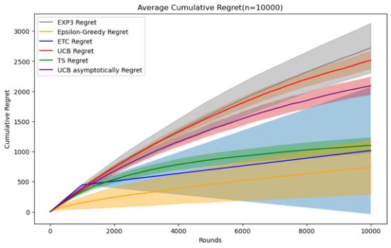
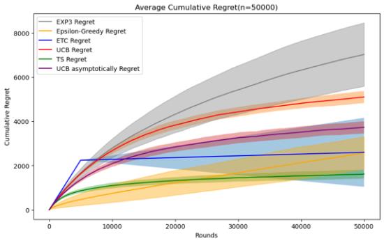
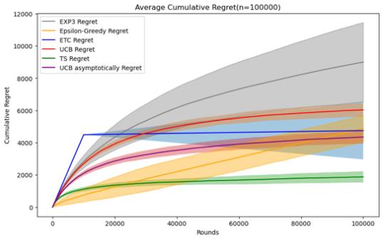
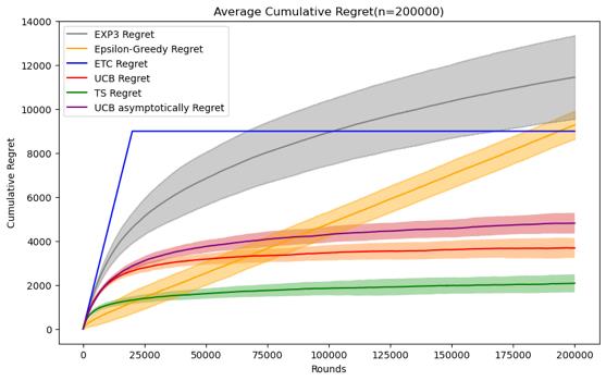
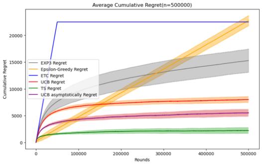
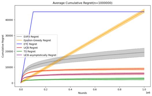
Figure 3. Cumulative regret comparison of five algorithms (Photo/Picture credit: Original).

By setting the number of experiments to 100 and designing a random number of seeds for each experiment, I tested five mainstream stochastic stationary bandits problem algorithms such as ETC, UCB, TS, epsilon-greedy, and EXP3 at n = 10000 and 50000. , 100000, 200000, 500000, 1000000, a graph of their average cumulative regret over time, and an error bar is set to observe their standard deviation, which can reflect the randomness of the algorithm under a given n situation and stability.

For these five algorithms, the parameters set respectively are ETC: m*k = 10%n, UCB: l = 4, epsilon-greedy: \( ϵ \) = 0.1, EXP3: \( γ= \sqrt[]{\frac{k*log{k}}{n}} \) , The TS algorithm follows the initialization process defined for normal algorithms, and in addition to these five algorithms, UCB asymptotically is added for comparison.

When the size of n is small, that is, when n=10000, 50000, the epsilon-greedy algorithm, ETC algorithm and TS algorithm perform better. When the number of n is 10000, the epsilon-greedy algorithm has an average cumulative regret. has the best performance, and the average cumulative regret of the ETC algorithm is also slightly smaller than that of the TS algorithm. The implementation methods of the two are also relatively simple, but it can be found that the randomness of the results of the epsilon greedy and ETC algorithms in this case is relatively large, and the variance Relatively high and when n = 50000, the TS algorithm is significantly better than several other algorithms. Therefore, when the number of n is small, you can give priority to the use of these three algorithms. Regarding the ranking of UCB, UCB asymptotically and EXP3 There is no change in these two cases of n. Since EXP3 is usually set as an algorithm in a special adversal environment, it does not perform well in this case, but it can also be seen from when n is small. It turns out that the UCB asymptotically algorithm is basically slightly better than the ordinary UCB1 algorithm.

As the number of n gradually increases to 100,000, the advantages of the TS algorithm gradually emerge. Its stability and average cumulative regret are both excellent. The advantages of the UCB algorithm can also be seen, especially UCB asymptotically. They gradually surpass the ETC algorithm and epsilon. -greedy algorithm, its advantages are mainly reflected in that the implementation method and operation speed are significantly better than the TS algorithm, and the stability is also similar to it. Currently, the average cumulative regret of the epsilon-greedy algorithm and the ETC algorithm are relatively close, but the values ​​of both are the performance has risen to a state where the performance is not good enough, and the standard deviation of the two is also larger than other algorithms.

When the number of n increases to more than 200,000, we can clearly see the differences between several algorithms, because their error bars overlap less and less. It is worth mentioning that although the EXP3 algorithm still has disadvantages in this case, due to its The characteristics of logarithm regret, when the number of n is large enough, the average cumulative regret has good performance. The TS and UCB algorithms still maintain a low average cumulative regret, and there is a convergence process similar to the ETC algorithm, indicating that they gradually The best arm was found and repeatedly selected through its own strategy. The average cumulative regret of the ETC algorithm and the epsilon-greedy algorithm did not perform well enough. However, the standard deviation of the ETC algorithm almost disappeared, indicating that the experimental results were almost stable.

Therefore, it can be concluded that without considering the time complexity and implementation difficulty of the algorithm, in the horizontal setting, the TS algorithm performs well enough in the stochastic bandits problem. The performance of the UCB algorithm is generally good. It is worth mentioning that its time complexity and implementation difficulty are better than those of the TS algorithm. When n is small, the ETC algorithm and the epsilon-greedy algorithm are worth trying, but there is also the problem of large standard deviation. EXP3 does not perform well enough when n is small, but as n increases, it can also reflect the characteristics of logarithm regret like TS UCB and other algorithms. Maybe it can perform better in specific environments.

3.1.2 Parameter Analysis and Optimization

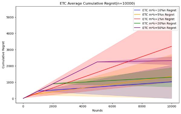
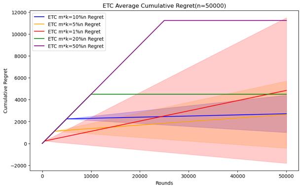
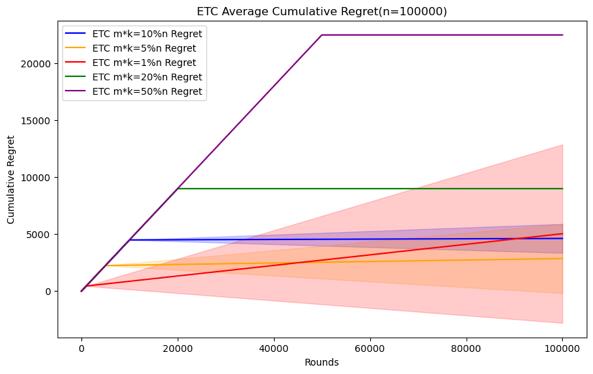
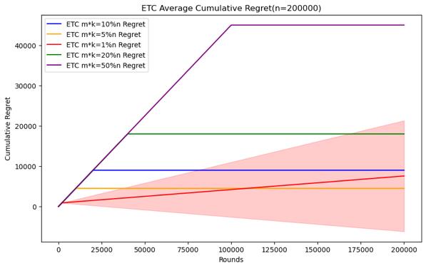
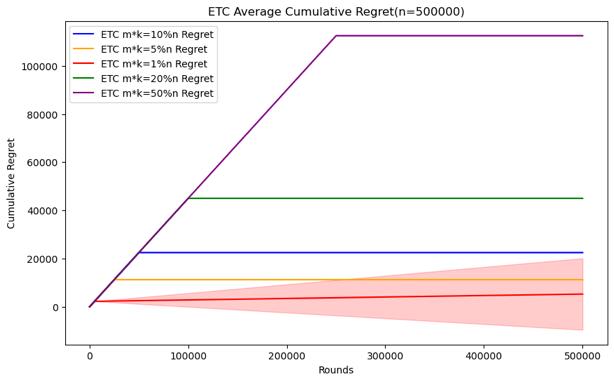
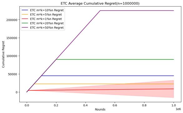
Figure 4. Cumulative regret comparison of ETC algorithms for different parameters (Photo/Picture credit: Original).

As shown in Figure 4.Regarding the ETC algorithm, it can clearly see the difference between the exploration and utilization stages in the experiment. Its purpose is to conduct random sampling in the exploration stage and continuously select the arm with the highest average value in the exploration stage in the utilization stage. The researcher is given In the case of horizon, the parameter that can be changed is m, and m*k is the length of the exploration phase. Therefore, the difficult problem is how to choose the length of the exploration phase under different horizon conditions. When setting n = 10000, 50000, 100000, 200000, 500000, 1000000, try to test m * k = 10%n, m * k = 5%n, m * k = 1%n, m * k = 20 %n, m * k = 50% performance of the ETC algorithm, the number of experiments is also 100.

When the scale of the horizon is small, the short exploration phase will cause it to not necessarily find the best arm in the utilization phase, and the standard deviation of the cumulative regret will be larger, indicating that the results are more random. This kind of In this case, although a more appropriate exploration phase length may not necessarily find the best arm or stabilize the experimental results, it can complete the appropriate and the optimization strategy for m mentioned above does not have a good effect. The longer The exploration phase will cause the accumulated regret to be too large, so it is necessary to establish the length of the exploration phase through experiments with different parameters. In the end, the accumulated regret, as the scale of the horizon increases, it can be seen that a relatively small exploration phase length can also be good To find the best arm and stabilize the experimental results, although there is still randomness in the minimum exploration phase length, it can achieve good performance, but the cumulative regret of the longer exploration phase is still too large, which can be used to make use of the previously mentioned The optimization strategy selects parameters, which can not only ensure that the cumulative regret is small, but also reduce the standard deviation.

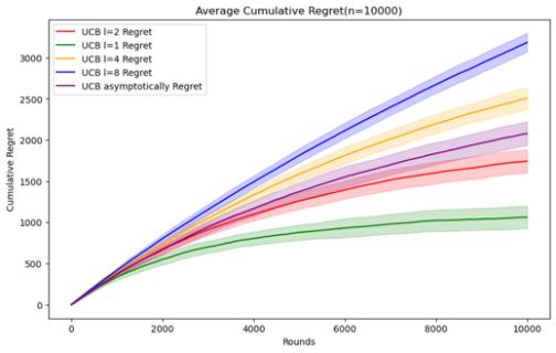
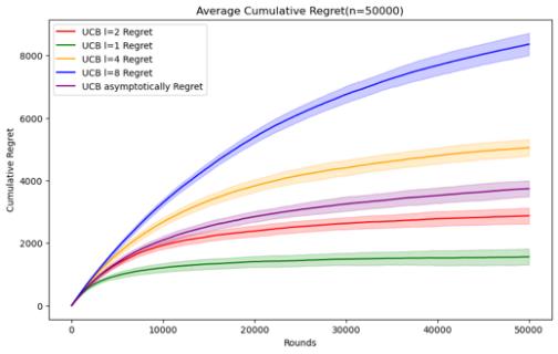
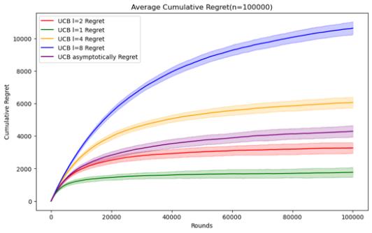
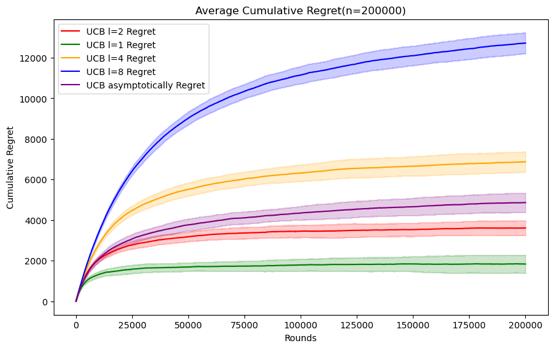
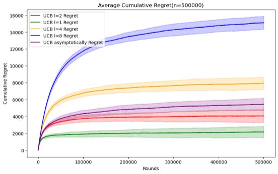
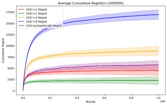
Figure 5. Cumulative regret comparison of UCB algorithms for different parameters (Photo/Picture credit: Original).

As shown in Figure 5.Regarding the UCB algorithm, the set parameters change to l = 1, 2, 4, 8 and UCB asymptotically, still using the n and data set mentioned above. When n = 50000, it can be seen that the UCB algorithm embodies the characteristics of logarithm regret. Within this range of n, the performance ranking of the UCB algorithm does not change significantly according to the parameters. Although it can be seen that UCB asymptotically is not significantly better than the UCB1 algorithm under the set parameters, but as n increases, It can be seen that UCB asymptotically is gradually approaching the situation of l = 2. When n=100000, the error bars of the two even intersect. Perhaps when n increases enough, UCB asymptotically can reflect the optimal situation.

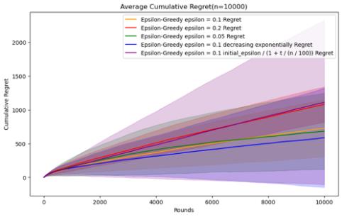
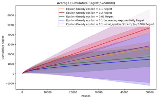
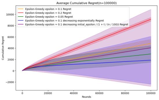
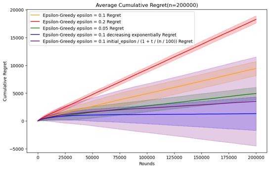
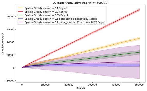
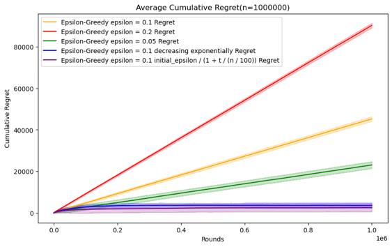
Figure 6. Cumulative regret comparison of epsilon-greedy algorithms for different parameters (Photo/Picture credit: Original).

As shown in Figure 6.For the epsilon-greedy algorithm, the parameters set are epsilon = 0.1, 0.2, 0.05 and epsilon decreases exponentially with time, and epsilon decreases reciprocally. When n is relatively small, there is no obvious cumulative regret gap under several parameter settings, and the error bars are also relatively large. For fixed epsilon, for this data set, epsilon = The performance of 0.05 will be slightly better than the other two, but if the value of epsilon is larger, it can be seen that the error bar is smaller, indicating that the experimental results are more stable. This may be because there are more opportunities to take advantage of instead of random selection.

As n increases, it can be seen that the parameter performance of epsilon as t decreases will be more advantageous, especially in the case of n = 500000. The two descent algorithms have superior performance. When n is small, as The average accumulated regret of the parameters of exponential decline will be better, and the stability of the parameters of reciprocal decline is relatively different. However, when n = 1000000, the performance of reciprocal decline is better than that of exponential decline. As shown in Figure 7.

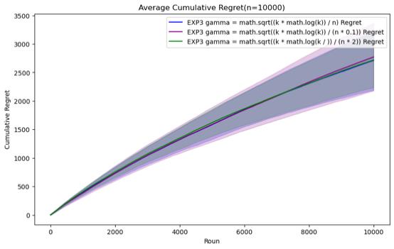
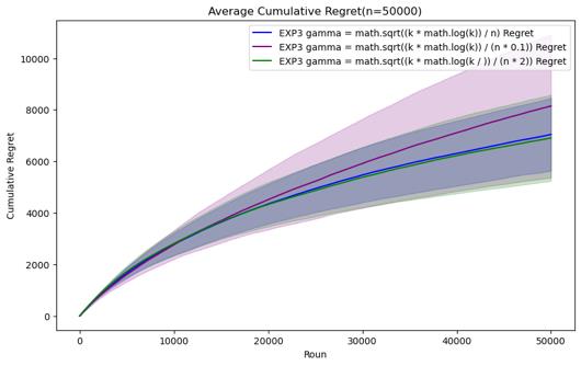
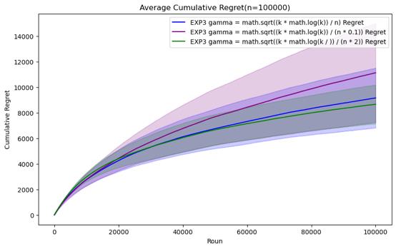
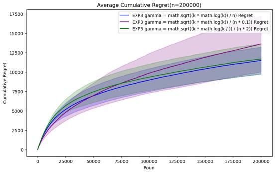
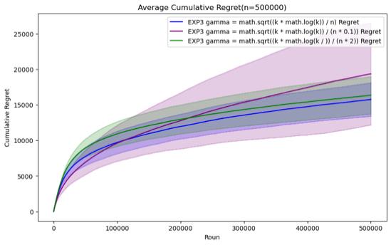
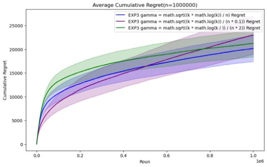
Figure 7. Cumulative regret comparison of EXP3 algorithms for different parameters (Photo/Picture credit: Original).

For the EXP3 algorithm, the set parameters are gamma = \( \sqrt[]{\frac{k*log{k}}{n}} \) , gamma = \( \sqrt[]{\frac{k*log{k}}{0.1*n}} \) and gamma = \( \sqrt[]{\frac{k*log{k}}{2* n}} \) . It can be seen that before n = 200000, Although there is not much difference in performance between the three parameter settings, gamma = \( \sqrt[]{\frac{k*log{k}}{0.1*n}} \) has certain advantages in those horizons. However, as n continues to increase, it is found that the performance of gamma = \( \sqrt[]{\frac{k*log{k}}{n}} \) gradually becomes the best. In the case of n=1000000, it can be clearly seen that its average cumulative regret exceeds other parameter settings.

3.2 Application in Diverse Fields

3.2.1 Recommendation Systems and Personalization. Regarding recommendation systems and personalization, it is one of the most widely used areas of MAB problems. Regarding recommendation systems and personalization, it is one of the most widely used areas of MAB problems. Current research on it mainly focuses on the recommendation of various streaming media. According to statistics, the top 10 are movies, news, synthetic, songs, products, genetics, ads, artists, jokes and POIs. Among the above algorithms, UCB and TS algorithms are more popular algorithms in this regard [3], which can also be seen through experimental results.

3.2.2 It is also more suitable to directly use the Stochastic Stationary Bandits problem algorithm than other problems. Research on such problems has also promoted various MAB Iteration and optimization of algorithms in problems. In new online platforms like ALEKS and TikTok, the MAB-A model and algorithms such as ULCB and KL-ULCB, which adjust exploration levels based on user feedback, effectively address the issue of user abandonment due to insufficient content engagement and significantly enhance the system's regret performance [4]. The challenge of mining user preferences is compounded by the large number of users and sparse interactions, and existing algorithms often overlook rich implicit feedback such as clicks and add-to-cart actions. Under these conditions, an algorithm named Dynamic Clustering-based Contextual Combinatorial Multi-Armed Bandit (DC (3) MAB) has been identified, which can improve performance [5]. In recommendation systems, there is a type of quantum greedy algorithm utilizing a quantum maximization approach, while the second is a simpler method that replaces the argmax operation in the ε-greedy algorithm with an amplitude encoding technique as a quantum subroutine. The results demonstrate that the performance of the quantum greedy algorithms in identifying the best arm is comparable to that of classical algorithms [6]. Regarding the impact of latent biases on rewards, suitable for recommendation systems that require the exclusion of factors such as race, a new model has been developed to optimize this strategy [7]. The CMAB model allows selecting multiple arms per round. The new AUCB algorithm, integrating UCB and auction theory, addresses arms' strategic behaviors and misinformation, ensuring authenticity and efficiency. The e-AUCB algorithm accommodates varying arm availability, with simulations confirming its significant performance [8].

3.2.3 Agriculture Decision-making. In agriculture, Multi-Armed Bandit (MAB) models are applied primarily to optimize decision-making and resource allocation. They assist in determining the best crop planting strategies by evaluating various crop types and varieties to maximize yield or minimize risk, managing irrigation by allocating water resources efficiently across different fields, controlling pests and diseases by choosing effective treatment methods at optimal times, and fine-tuning the use and application of fertilizers and pesticides to balance environmental sustainability with economic benefits. Through these applications, MAB models significantly enhance agricultural productivity and help farmers adapt to environmental changes and market risks, moving towards precision and smart agriculture.

A decision support system has been developed to diagnose post-harvest diseases in apples, leveraging multiple conversational rounds to gather user feedback. This system employs a contextual multi-armed bandit approach to dynamically adapt its image selection mechanism based on the feedback. Comparative studies with baseline strategies have shown that the exploration and exploitation principle greatly enhance the effectiveness of the image selection process [9]. Reinforcement learning (RL), particularly through multi-armed bandits (MAB), effectively tackles sequential decision-making in uncertain environments, crucial in fields like crop management decision support systems (DSS). MAB demonstrates RL's potential in dynamic and context-sensitive decision-making required for agricultural operations. Although its application in agriculture is emerging, there is significant potential for MAB to revolutionize crop management DSS by enhancing decision-making processes in the face of uncertainties. This underscores the need for collaborative research between the RL and agronomy communities to fully harness MAB's capabilities in agriculture [10].

3.2.4 Financial Investment Models. In the field of finance, multi-armed bandit (MAB) problems are applied to optimize the balance between expected returns and associated risks, particularly through the use of Conditional Value at Risk (CVaR). A novel set of distribution-oblivious algorithms has been developed to efficiently select financial portfolios within a fixed budget without needing prior knowledge of the reward distributions. These algorithms are complemented by a newly devised estimator for CVaR that can handle unbounded or heavy-tailed distributions, and a proven concentration inequality. Comparative analysis with standard non-oblivious algorithms demonstrates that the new approaches perform robustly, confirming the practical viability of applying MAB methods to enhance risk management in financial decision-making [11].

Thompson Sampling is adapted to handle rewards from symmetric alpha-stable distributions, a type of heavy-tailed probability distribution common in finance and economics for modeling phenomena like stock prices and human behavior. An efficient framework for posterior inference has been developed, leading to two Thompson Sampling algorithms specifically tailored for these distributions. Finite-time regret bounds have been proven for both algorithms, and experimental results demonstrate their superior performance in handling heavy-tailed distributions. This approach facilitates sequential Bayesian inference and enhances decision-making in financial and complex systems characterized by heavy-tailed features [12].

3.2.5 Clinical Trial Methodologies. In clinical trials, the approach to the multi-armed bandit problem incorporates safety risk constraints where each arm represents a different trial strategy with unknown safety risks and rewards. The goal is to maximize rewards while adhering to safety standards, defined by a set threshold for mean risk per round, ensuring continuous patient safety rather than cumulative evaluation. The strategy involves doubly optimistic indices for both safety and rewards, leading to tight gap-dependent logarithmic regret bounds and minimizing unsafe arm plays to logarithmically many times. Simulation studies confirm the effectiveness of these strategies in maintaining stringent safety measures in clinical trials [13].

Clinical trials utilizing multiple treatments often employ randomization to assess treatment efficacies, which can lead to suboptimal outcomes as participants may not receive the most suitable treatments. Reinforcement-learning methods, specifically multi-arm bandits, offer a dynamic way to learn and adapt treatment assignments during trials. The contextual-bandit algorithm optimizes treatment decisions based on clinical outcomes and patient characteristics, enhancing the precision of treatment assignments. In simulations using data from the International Stroke Trial, this method significantly outperformed both random assignment and a context-free multi-arm bandit approach, demonstrating substantial improvements in assigning the most appropriate treatments to participants [14].

4 Challenges

Despite the effectiveness of Multi-Armed Bandit (MAB) algorithms in optimizing decision-making in uncertain environments, they face several practical challenges. These include the complexity of tuning parameters, adapting to dynamically changing environments, computational resource constraints, scalability issues with many options, ethical considerations and bias mitigation, and the intricacies of multi-objective optimization. Overcoming these challenges necessitates ongoing algorithmic innovation, improved parameter optimization techniques, and tailored solutions for specific application domains. The stochastic stationary problem is only one of the most basic categories of MAB problems. If it is to be connected to practical applications such as recommendation systems or to the classification of other MAB problems, researchers still need to make more iterative updates and explore it.

5 Conclusions

This study presents a detailed examination of stochastic stationary multi-armed bandit algorithms, analyzing their deployment and relative efficacy across varied datasets characterized by different attributes. Through meticulous evaluation of algorithms such as Explore-then-Commit, Upper Confidence Bound, Thompson Sampling, epsilon-greedy, and EXP3, this research delineates the performance contours of these methodologies under assorted conditions, thereby deepening insights into their practical utility in domains including recommendation systems and clinical trials. The results emphasize the criticality of selecting appropriate algorithms based on specific environmental factors and underscore the necessity for continued research to tackle issues like dynamic settings, scalability, and computational demands. Such efforts are essential to refine these decision-making tools for effective real-world application.

References

[1]. Matsuo, Y., LeCun, Y., Sahani, M., Precup, D., Silver, D., Sugiyama, M., Uchibe, E., & Morimoto, J. (2022). Deep learning, reinforcement learning, and world models. Neural Networks, 152, 267–275. https://doi.org/10.1016/j.neunet.2022.03.037.
[2]. Afsar, M. M., Crump, T., & Far, B. (2022). Reinforcement Learning based Recommender Systems: A Survey. ACM Comput. Surv., 55(7). https://doi.org/10.1145/3543846.
[3]. Silva, N., Werneck, H., Silva, T., Pereira, A. C. M., & Rocha, L. (2022). Multi-Armed Bandits in Recommendation Systems: A survey of the state-of-the-art and future directions. Expert Systems with Applications, 197, 116669. https://doi.org/10.1016/j.eswa.2022.116669.
[4]. Yang, Z., Liu, X., & Ying, L. (2024). Exploration, Exploitation, and Engagement in Multi-Armed Bandits with Abandonment. Journal of Machine Learning Research, 25(9), 1–55. http://jmlr.org/papers/v25/22-1251.html.
[5]. Yan, C., Han, H., Zhang, Y., Zhu, D., & Wan, Y. (2022). Dynamic clustering based contextual combinatorial multi-armed bandit for online recommendation. Knowledge-Based Systems, 257, 109927. https://doi.org/10.1016/j.knosys.2022.109927.
[6]. Ohno, H. (2023). Quantum greedy algorithms for multi-armed bandits. Quantum Information Processing, 22(2), 101. https://doi.org/10.1007/s11128-023-03844-2.
[7]. Kang, Q., Tay, W. P., She, R., Wang, S., Liu, X., & Yang, Y.-R. (2024). Multi-armed linear bandits with latent biases. Information Sciences, 660, 120103. https://doi.org/10.1016/j.ins. 2024. 120103.
[8]. Zhu, X., Huang, Y., Wang, X., & Wang, R. (2023). Emotion recognition based on brain-like multimodal hierarchical perception. Multimedia Tools and Applications, 1-19.
[9]. Sottocornola, G., Nocker, M., Stella, F., & Zanker, M. (2020). Contextual multi-armed bandit strategies for diagnosing post-harvest diseases of apple. Proceedings of the 25th International Conference on Intelligent User Interfaces, 83–87. https://doi.org/10.1145/3377325.3377531.
[10]. Gautron, R., Maillard, O.-A., Preux, P., Corbeels, M., & Sabbadin, R. (2022). Reinforcement learning for crop management support: Review, prospects and challenges. Computers and Electronics in Agriculture, 200, 107182. https://doi.org/10.1016/j.compag.2022.107182.
[11]. Kagrecha, A., Nair, J., & Jagannathan, K. P. (2019, December). Distribution oblivious, risk-aware algorithms for multi-armed bandits with unbounded rewards. In NeurIPS (pp. 11269-11278).
[12]. Dubey, A., & Pentland, A. (2019). Thompson Sampling on Symmetric $\alpha $-Stable Bandits. arXiv preprint arXiv:1907.03821.
[13]. Chen, T., Gangrade, A., & Saligrama, V. (2022, June). Strategies for safe multi-armed bandits with logarithmic regret and risk. In International Conference on Machine Learning (pp. 3123-3148). PMLR.
[14]. Varatharajah, Y., & Berry, B. (2022). A Contextual-Bandit-Based Approach for Informed Decision-Making in Clinical Trials. Life, 12(8). https://doi.org/10.3390/life12081277.
Cite this article
Song,R. (2024). Optimizing decision-making in uncertain environments through analysis of stochastic stationary Multi-Armed Bandit algorithms. Applied and Computational Engineering,68,93-113.
Data availability
The datasets used and/or analyzed during the current study will be available from the authors upon reasonable request.
Disclaimer/Publisher's Note
The statements, opinions and data contained in all publications are solely those of the individual author(s) and contributor(s) and not of EWA Publishing and/or the editor(s). EWA Publishing and/or the editor(s) disclaim responsibility for any injury to people or property resulting from any ideas, methods, instructions or products referred to in the content.
About volume
Volume title: Proceedings of the 6th International Conference on Computing and Data Science
© 2024 by the author(s). Licensee EWA Publishing, Oxford, UK. This article is an open access article distributed under the terms and
conditions of the Creative Commons Attribution (CC BY) license. Authors who
publish this series agree to the following terms:
1. Authors retain copyright and grant the series right of first publication with the work simultaneously licensed under a Creative Commons
Attribution License that allows others to share the work with an acknowledgment of the work's authorship and initial publication in this
series.
2. Authors are able to enter into separate, additional contractual arrangements for the non-exclusive distribution of the series's published
version of the work (e.g., post it to an institutional repository or publish it in a book), with an acknowledgment of its initial
publication in this series.
3. Authors are permitted and encouraged to post their work online (e.g., in institutional repositories or on their website) prior to and
during the submission process, as it can lead to productive exchanges, as well as earlier and greater citation of published work (See
Open access policy for details).