1.Introduction

With the advent of the Internet era, for banks in major financial systems, credit loans have brought great convenience, but at the same time, there are also some inevitable potential crises. The increase in credit loan problems over a short period of time in previous years was at the heart of the crisis in most financial institutions [1]. Most banks in the financial industry focus on credit risk due to the global economic crisis from 2007 to 2008 [2]. The financial industry uses forecasting methods to reduce the risk of credit risk. Financial companies begin to accurately assess risks to utilize resources more efficiently [3]. The financial sector uses algorithms and risk-based financial models for forecasting to combat credit risk. Model performance is used in most consumer lending to evaluate whether to grant a loan, in the financial sector [1]. This article will use machine learning methods to predict whether the borrower will have credit loan risk for bank based on characteristics of the borrower. We solve this problem by using XGBoost method. In this paper, we will build a XGBoost model to predict credit loan risk. The rate of receiver operating characteristic curve (ROC) is 0.87 and the rate of Kolmogorov-Smirnov test (KS) is 0.56. We realized there was development for improvement in this machine learning model. The result of paper is recognised as follows. Section 2 describes the literature review. Whereas, Section 3 shows methodology. Section 4 represents the experimental results and their analysis. The last Section presents a summary of this paper.

2.Literature Review

Some scholars use machine learning technology to predict the risk of defaulting on credit loans. Ali et al. predict the risk of late repayments on a credit loan by applying a variety of machine learning techniques including variations of artificial neural networks, ensemble classifiers, and decision trees [1]. They finally find that Artificial Neural Network-Multilayer Perceptron (ANN-MLP) is a useful tool to handle the risk for bank which has more benefits than using traditional binary logistic regression technique. However, Xu et al. using borrower characteristics such as asset status, industry development, profitability, and working capital turnover studied that the random forest model can identify default objects well through the feature importance analysis of the model by methods including random forest, extreme gradient boosting tree, gradient boosting model and neural network [4]. For other scholars have different opinions about the methods. Decision trees have more accurate predictions compared to k-nearest neighbors and neural networks [3]. Ensemble technologies may hold better prospects. Each model has its own risks and challenges, and ensemble techniques perform better than single classifiers [2].

3.Methodology

3.1.XGBoot Model establishment and application

3.1.1.XGBoot Model establishment

XGBoost(Extreme Gradient Boosting)is a powerful gradient boosting machine learning algorithm that builds a strong model by iteratively training multiple weak learners (Usually it is decision tree), each iteration stage corrects the error of the previous stage model.

Figure 1. Modeling Building

3.1.2.Objective function

The core of XGBoost is to define an objective function, which needs to be minimized. The objective function consists of two parts: loss function and regularization term

*Objective function = loss function + regularization term

\( Obj(ϕ)=L(ϕ)+Ω(ϕ) \)

Include

\( ϕ=\lbrace {ω_{i}}|i=1,2,3,…,d\rbrace \)

*Loss function: used to measure the difference between the model’s predicted value and the actual label.

\( L=\sum _{i=1}^{n}l({y_{i}},\hat{{y_{i}}}) \)

* Regularization term: used to prevent model overfitting. XGBoost uses L1 (Lasso regularization) and L2 (Ridge regularization) regularization terms. GBoost's regularization term helps control the complexity of the tree. At each iteration, a regularization term is added to the objective function to prevent the tree from growing too deep or too complex.

L1(Lasso Regularization)

\( Ω(ω)=λ{||ω||_{1}} \)

L2(Ridge Regularization)

\( Ω(ω)=λ{||ω||^{2}} \)

3.1.3.Iterations of Gradient Boosting

XGBoost uses the gradient boosting method to update the model by calculating the gradient of the loss function (the gradient represents the error of the current model for each sample, or the derivative of the loss function relative to the parameters of the model). For classification tasks (log loss):

Loss function:

\( L(y,p)=-[y*log{(p)}+(1-y)*log{(1-p)}] \)

The gradient of the loss function on the model output:

\( \frac{∂L}{∂F(x)}=p-y \)

y is the true label, F(x) is the predicted output of the current model, and p is the model’s probability estimate.

4.Experimental results and their analysis

This part, following an initial exploratory analysis of the Give Me Some Credit dataset on Kaggle (Give Me Some Credit | Kaggle), undertakes data cleansing and variable selection. The data is partitioned into training, validation, and test sets. To address the class imbalance issue within the training set, the positive samples are randomly divided into five equal portions and combined with the negative samples, resulting in five new training sets. This approach aims to reduce the severity of class imbalance within each training subset.

4.1.Experimental Data

This paper will prove the superiority of this model through a series of experimental evaluation indicators. This experimental dataset is from a project launched in Kaggle (Give Me Some Credit | Kaggle), which includes 11 indicators. The column index English name of the dataset along with their meanings are shown in the following table.

Table 1. The column index English name of the dataset along with their meanings

The above table discusses a total of 11 indicators, with "SeriousDlqin2yrs" serving as an indicator for whether a borrower has experienced a loan delinquency. The remaining 10 indicators represent dependent variables used in this project to assess whether a borrower has experienced a loan delinquency. This dataset comprises 150,000 rows of data.

4.2.Dataset dimension partitioning

A first look at the training dataset, with 150,000 rows of data. A preliminary review found a total of 609 data duplicates. After the duplicate value is deleted, 149391 rows of data remain.

In addition to “SeriousDlqin2yrs” as an indicator of whether the borrower is overdue, the remaining 10 indicators can be divided into the following four dimensions: personal information, repaying capability, credit standing, debt situation. Figure 2 shows the detailed categories.

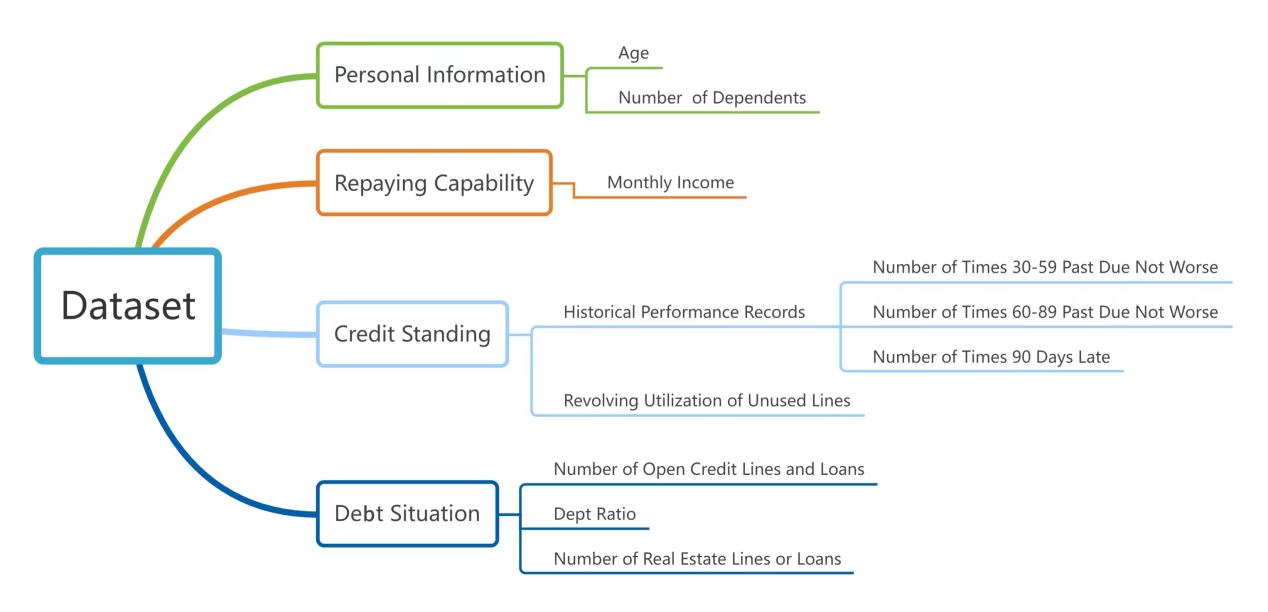
Figure 2. Dataset dimension partitioning

4.3.Data visualization

Through python, the dataset was presented by different graphs such as histograms, box plots, and heat map. The results will be shown as follows.

4.3.1.Personal information

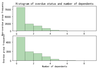
Figure 3. Histogram of overdue status and number of dependents

From Figure 3, there’s no obvious correlation between the number of dependents and overdue status.

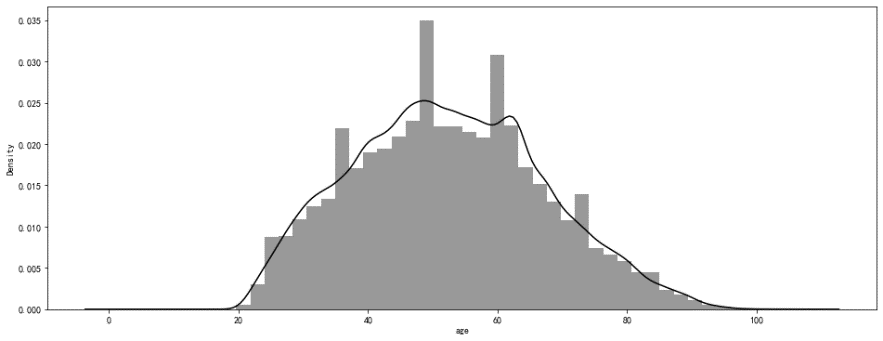
Figure 4. Normal distribution of sample age

As can be seen from Figure 4, the sample age basically conforms to the normal distribution.

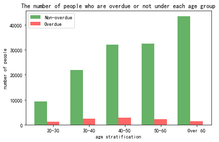
Figure 5. Histogram of the number of people who are overdue or not under each age group

From Figure 5 above, it is evident that the older the individuals are, the greater the number of non-delinquent cases. Those aged 60 and above constitute the largest demographic of non-delinquent individuals, whereas the age group between 40 and 50 years exhibits the highest number of delinquent cases. Additionally, when examining the delinquency rate, it becomes apparent that the probability of experiencing delinquency decreases as individuals grow older.

4.3.2.Repaying capability

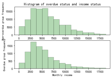
Figure 6. Histogram of overdue status and income status

As can be seen in Figure 6, it is evident that the income range for individuals with delinquencies primarily falls within the range of 2500 yuan to 3725 yuan, while those without delinquencies tend to have their income concentrated in the range of 2500 yuan to 6250 yuan.

4.3.3.Credit standing

4.3.3.1.Historical performance records

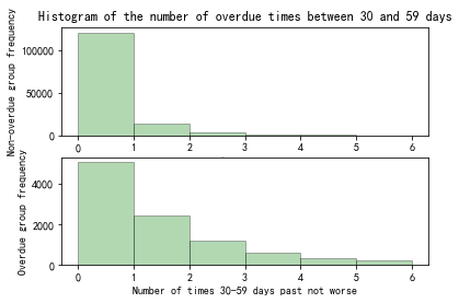
Figure 7. Histogram of the number of overdue times between 30 and 59 days

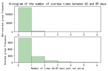
Figure 8. Histogram of the number of overdue times between 60 and 89 days

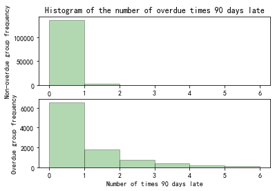
Figure 9. Histogram of the number of overdue times 90 days late

Within the historical performance records of the overdue group, shown in Figure 7 to Figure 9, the proportion of occurrences of overdue is greater than the proportion in the non-overdue group.

4.3.3.2.Revolving utilization of used lines

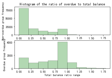
Figure 10. Histogram of the ratio of overdue to total balance

According to Figure 10, it can be seen that in the overdue group, the higher the total balance, the larger the proportion.

4.3.4.Debt situation

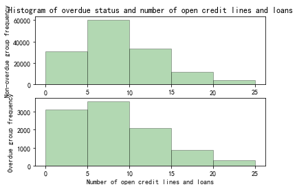
Figure 11. Histogram of overdue status and open credit lines and loans

From Figure 11, there’s no obvious correlation between the number of outstanding loans and lines of credit, and overdue status.

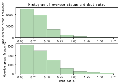
Figure 12. Histogram of overdue status and debt ratio

From Figure 12, it can be observed that within the debt ratio range of 0.5 to 1.75, the overdue group's proportion of individuals is slightly greater compared to the non-overdue group.

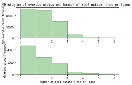
Figure 13. Histogram of overdue status and number of real estate lines or loans

From Figure 13, it can be seen that the proportion of people in the overdue group who have 1 or 2 sets of mortgages is smaller than that of the non-overdue group. That is, the probability of overdue borrowers with mortgages and real estate as security is smaller than that of borrowers without mortgages and real estate as security.

In summary, it can be preliminarily seen that variables in personal information such as age, repaying capability, number of mortgage loans in debt situation, and credit status can predict whether the borrower will be overdue in the future.

4.4.Data cleaning

4.4.1.Missing value handling

Missing values are found in the columns of monthly income and number of dependents. In order to handle this, the number of dependents is filled with its mode while the missing value of monthly income are deleted.

4.4.2.Outlier processing

After processing the missing values, using the box plot shown in Figure 14, it can be found that the difference between the maximum value of the remaining amount, debt ratio and personal income and the average value is too large, which is obviously greater than the average value +3 standard deviations. Due to the large value of the outlier, the average value is too close to the X-axis on the Y-axis. Some values of age, the number of outstanding loans, and the number of family members are greater than the upper limit of the box plot, but the numerical differences are not too great. There are obvious outliers for 30-59 days, 60-89 days and 90 days overdue. These results have been illustrated in Table 2.

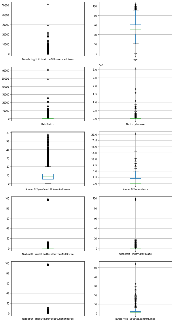
Figure 14. Box plot

Table 2. Outlier processing result

4.5.Variable selection

The Pearson correlation coefficient is used to prevent the linear correlation between variables. If the coefficient is greater than 0.6, the redundant variables with high correlation need to be deleted.

According to Figure 15, the coefficient is between each variables are less than 0.6, so there is no variable has to be deleted.

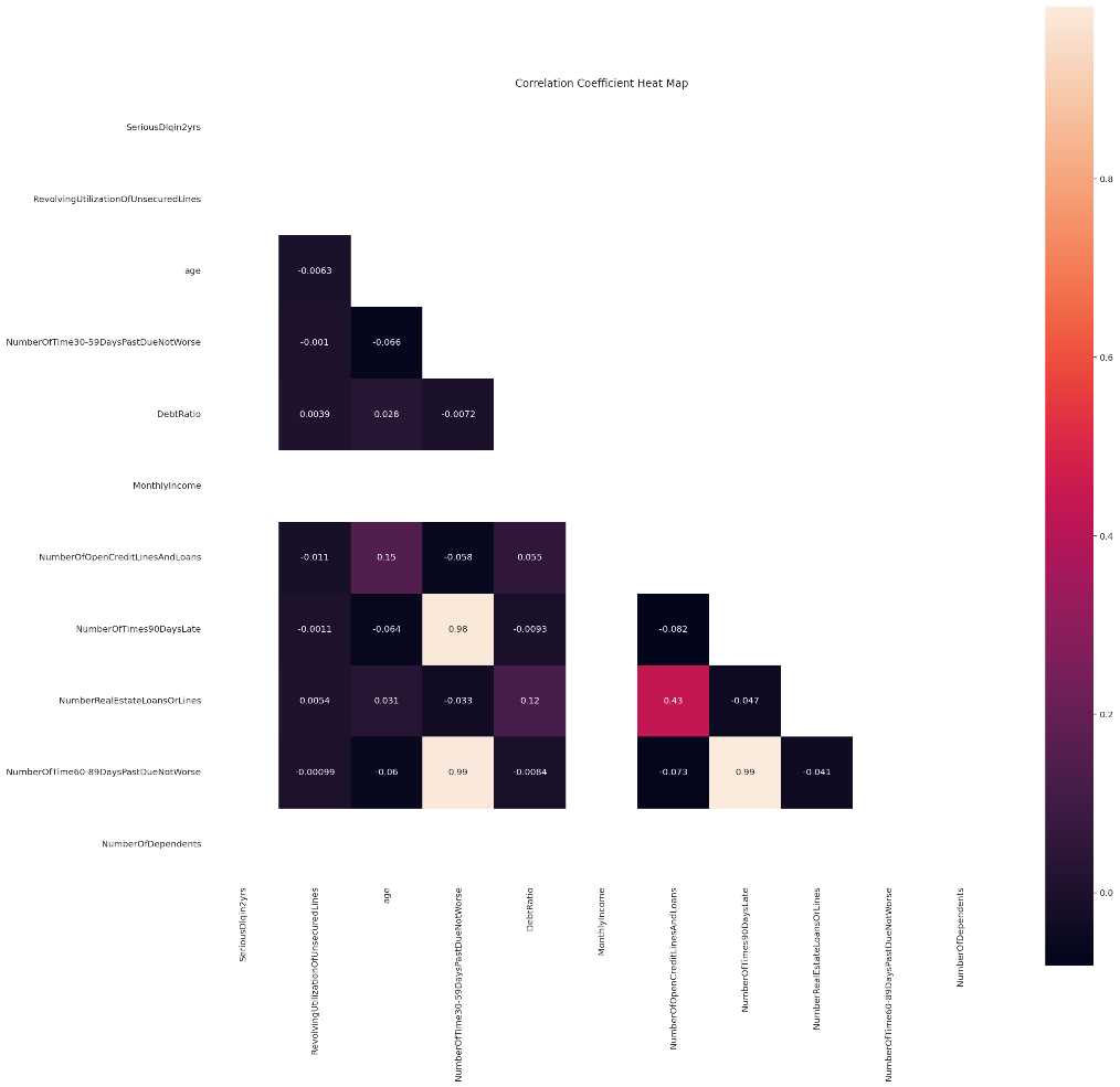
Figure 15. Correlation Coefficient Heat Map

5.XGBoost Model application [5]

5.1.The reason for selecting the XGBoost model

We need to classify the features. There are many methods. In order to achieve the optimal feature classification, we use these methods to obtain the cv value through python (CV is the coefficient of variation, which is the ratio of the standard deviation to the average value in percentage. Finally we choose XGBoost for feature classification.

Table 3. CV-Means of different methods

5.2.Model optimization and parameter adjustment

(1) learning_rate:A large learning rate gives greater weight to the contribution of each tree in the ensemble, but this may lead to overfitting/instability and speed up training time. While a lower learning rate suppresses the contribution of each tree, making the learning process slower but more robust. This regularizing effect of the learning rate parameter is particularly useful for complex and noisy data sets.

(2) max_depth:maximum depth (max_depth) controls the maximum number of levels a decision tree may reach during training. Deeper trees can capture more complex interactions between features. However, deeper trees also have a higher risk of overfitting because they can remember noise or irrelevant patterns in the training data. To control this complexity, we can limit max_depth result in shallower, simpler trees that capture more general patterns. The Max_depth value provides a good balance between complexity and generalization.

(3) alpha, lambda:alpha (L1) and lambda (L2) are two regularization parameters that help overfitting.

The difference from other regularization parameters is that they can reduce the weight of unimportant or unimportant features to 0 (especially alpha), resulting in a model with fewer features and thus reduced complexity. The result of Alpha and lambda may be affected by other parameters such as max_depth､subsamplean and colsample_bytree. Higher alpha or lambda values may require adjusting other parameters to compensate for the increased regularization.

Final parameter result:

Table 4. Parameter values

6.Model testing

6.1.ROC curves

Coefficient: 0.87

The ROC curve coefficient is one of the important indicators to measure the classification accuracy of the model. Its value range is between 0 and 1. The closer it is to 1, the stronger the classification ability of the model. The ROC curve coefficient of 0.86 shows that the model has a good ability to distinguish between positive and negative examples. This means that the model can accurately distinguish positive examples from negative examples and can maintain a high true positive rate and a low false positive rate under different thresholds. This result shows that the model has high prediction accuracy and reliability and can provide valuable prediction results in classification tasks.

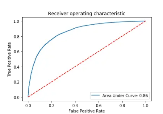
Figure 16. Receiver operating characteristic

6.2.KS curves

Coefficient: 0.56

The KS curve coefficient is one of the important indicators to measure the discrimination of the model. Its value range is between 0 and 1. The closer to 1, the better the discrimination of the model. In this case, the Figure 17 shows the KS curve coefficient of 0.56 indicates that the model is good at distinguishing between positive and negative examples, but not very strong. This means that the model can distinguish positive and negative examples to a certain extent, but there is room for improvement.

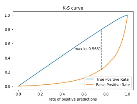
Figure 17. K-S curve

7.Conclusion

7.1.Summary

This paper conducts an in-depth analysis of credit risk in financial institutions, employing machine learning techniques to assess the credit risk based on borrower characteristics. The study demonstrates that the Extreme Gradient Boosting (XGBoost) model outperforms traditional methods such as KNN, Random Forest, and Logistic Regression in accurately identifying credit risks. After data pre-processing the "Give Me Some Credit" dataset from Kaggle, which involved data cleansing, variable selection, partitioning, and addressing class imbalance, the XGBoost model was applied, resulting in a ROC curve coefficient of 0.87 and a KS curve coefficient of 0.56. These results indicate the model's proficiency in distinguishing between positive and negative samples, albeit with room for improvement.

7.2.Future Works

Future work could enhance this research from several perspectives: Firstly, exploring more feature engineering techniques and data pre-processing methods could improve model performance. Secondly, given the potential of different models to excel in specific scenarios, employing model ensemble techniques to combine the strengths of various machine learning models could further increase predictive accuracy. Additionally, to enhance the model's generalizability, testing and validating the model on a broader and more diverse dataset is recommended. Through the exploration and implementation of these approaches, the predictive capability of the model regarding credit risk can be further strengthened, providing more reliable decision support for financial institutions.

Acknowledgments

Wenhao Wang, Xiyi Zuo, Dantong Han, which authors contributed to the work equally and should be regarded as co-first authors.

References

[1]. Ali, SEA, Rizvi, SSH, Lai, F, Ali, RF & Jan, AA (2021), Predicting Delinquency on Mortgage Loans: An exhaustive parametric comparison of machine learning techniques, International Journal of Industrial Engineering and Management [online] 12(1):pp.1–13. Available at: https://doi.org/10.24867/ijiem-2021-1-272 [Accessed 10 October 2023].
[2]. Bhatore, S, Mohan, S & Reddy, YR (2020) Machine learning techniques for credit risk evaluation: a systematic literature review, Journal of Banking and Financial Technology, [online] 4(1):pp.111–138. Available at: https://doi.org/10.1007/s42786-020-00020-3 [Accessed 10 October 2023].
[3]. Galindo, JF & Tamayo, P (2000), Credit Risk Assessment Using Statistical and Machine Learning: Basic Methodology and Risk Modeling Applications, Computational Economics [online] 15(1/2):pp.107–143, Available at: https://doi.org/10.1023/a:1008699112516 [Accessed 10 October 2023].
[4]. Xu, J., Lu, Z. and Xie, Y. (2021) Loan default prediction of Chinese P2P market: A machine learning methodology. Scientific Reports [online] 11(1) Available at: https://dx.doi.org/10.1038/s41598-021-98361-6 [Accessed 10 October 2023].
[5]. Zhang, F., Jing, Y., Guo, Y. Q., & Gu, H. (2020). Multi-source heterogeneous and XBOOST vehicle sales forecasting model. In Advances in intelligent systems and computing [online] pp. 340–347, Available at: https://doi.org/10.1007/978-3-030-62746-1_50 [Accessed 20 October 2023]
Cite this article
Wang,W.;Zuo,X.;Han,D. (2024). Predict credit risk with XGBoost. Applied and Computational Engineering,74,164-177.
Data availability
The datasets used and/or analyzed during the current study will be available from the authors upon reasonable request.
Disclaimer/Publisher's Note
The statements, opinions and data contained in all publications are solely those of the individual author(s) and contributor(s) and not of EWA Publishing and/or the editor(s). EWA Publishing and/or the editor(s) disclaim responsibility for any injury to people or property resulting from any ideas, methods, instructions or products referred to in the content.
About volume
Volume title: Proceedings of the 2nd International Conference on Software Engineering and Machine Learning
© 2024 by the author(s). Licensee EWA Publishing, Oxford, UK. This article is an open access article distributed under the terms and
conditions of the Creative Commons Attribution (CC BY) license. Authors who
publish this series agree to the following terms:
1. Authors retain copyright and grant the series right of first publication with the work simultaneously licensed under a Creative Commons
Attribution License that allows others to share the work with an acknowledgment of the work's authorship and initial publication in this
series.
2. Authors are able to enter into separate, additional contractual arrangements for the non-exclusive distribution of the series's published
version of the work (e.g., post it to an institutional repository or publish it in a book), with an acknowledgment of its initial
publication in this series.
3. Authors are permitted and encouraged to post their work online (e.g., in institutional repositories or on their website) prior to and
during the submission process, as it can lead to productive exchanges, as well as earlier and greater citation of published work (See
Open access policy for details).